Tracing Itineraries in the State Papers

This is an R Notebook: a document containing code and text. The source code is available in a GitHub repository: download the folder and then open it with R-Studio to run the notebook yourself. You’ll need a little bit of prior knowledge of R and the tidyverse to properly follow along. This post is the second in a series documenting some of the code and techniques we’ve been using on the Networking Archives project: you can read the first one, looking at Wikidata, here.

More info on the Github repository below

Geographic Data and the Stuart State Papers

The Stuart State Papers are a treasure trove of geographic data: on the Networking Archives project we have found coordinates for the origins of more than 80,000 letters in the dataset. These letter origins can be plotted as points on a map, giving an overview of the key places from where correspondence we being sent, but there are other ways to represent and analyse the dataset spatially.

Many of the individuals in the data do not just send multiple letters from the same spot, but rather travel around for various reasons, sending letters, often at great expense, back to government officials in London. In the seventeenth century, letter authors might travel as part of a diplomatic mission, or as part of a ‘grand tour’, or, in some cases, because they were forcibly displaced or exiled. In the State Papers are found, for example, individuals displaced by the English Civil War: many leading politicians and generals were exiled to the continent following the defeat of the Royalists and the execution of Charles I in January 1649. As they would have been at the time they were written, the letters in the State Papers are an excellent source of news about events and places, and for understanding more about life on the move in early modern Europe.

Reconstructing Itineraries

We can use the the points of origin of the letters to reconstruct parts of these routes or itineraries.The basic method to do this is to line up all the origins from where a given individual wrote a letter, then draw a line connecting them in date order. The resulting line can be used for a whole host of spatial operations. All this can be done with the R package ‘sf’. This package is very fast, relatively easy to use, and completely free, so no need for any expensive licensed GIS software.

In this post I’m going to show how to use the sf package to create a geographic object, transform each individual’s origin locations into a single line, measure those lines, and then map one, before introducing some basic spatial computation. The object used to do all this is created through the following steps:

Import places data
Join the letter places to the coordinates table
Turn into a sf object
Summarise by each person
Cast to a linestring

Import places data

First, we need place data. I’ve made a very simplified sample of the State Papers data with which to work. It contains just the necessary info we need to measure journeys. The data is divided into three tables, which will be joined together when needed. I’ve saved them as the following tables:

First, the main letters table, called sp_letters. This contains the letter records for the sample. It has an ID for each person, the date of the letter, and the origin.

library(tidyverse)  
sp_letters = read_csv('/Users/Yann/Documents/Github/blog_notebooks/sp_letters.csv')

glimpse(sp_letters)

## Rows: 3,346
## Columns: 3
## $ person_id  <dbl> 22662, 22662, 13045, 22662, 13045, 22662, 30822, 42044, 43…
## $ date       <dbl> 16030330, 16030412, 16030704, 16030710, 16030912, 16031001…
## $ place_name <chr> "London", "London", "Windsor", "London", "Eaglefield", "Hi…

Next, a lookup table containing the ID code for each person in the sample, plus their actual name:

sp_people = read_csv('/Users/Yann/Documents/Github/blog_notebooks/sp_people.csv')
glimpse(sp_people)

## Rows: 99
## Columns: 2
## $ person_id   <dbl> 13045, 7154, 22662, 42773, 30822, 42044, 43109, 51384, 41…
## $ person_name <chr> "Dudley Carleton, Viscount Dorchester", "Charles, Viscoun…

Last, a lookup table containing the coordinates for each place:

sp_coords = read_csv('/Users/Yann/Documents/Github/blog_notebooks/sp_coords.csv')
glimpse(sp_coords)

## Rows: 459
## Columns: 3
## $ place_name            <chr> "Abergavenny", "Aboard the Assurance at Lee", "…
## $ coordinates_latitude  <dbl> -3.0172222, 0.6500000, 9.2844444, 9.2844444, 9.…
## $ coordinates_longitude <dbl> 51.833056, 51.550000, 53.823056, 53.823056, 53.…

Join the letters to the coordinates table

Next, we join the sp_coords table to the sp_letters table, using the ‘place_name’ column. This will add the coordinates for each place.

sp_letters_with_coordinates = sp_letters %>% left_join(sp_coords, by = 'place_name')

glimpse(sp_letters_with_coordinates)

## Rows: 3,346
## Columns: 5
## $ person_id             <dbl> 22662, 22662, 13045, 22662, 13045, 22662, 30822…
## $ date                  <dbl> 16030330, 16030412, 16030704, 16030710, 1603091…
## $ place_name            <chr> "London", "London", "Windsor", "London", "Eagle…
## $ coordinates_latitude  <dbl> -0.1275000, -0.1275000, -0.6000000, -0.1275000,…
## $ coordinates_longitude <dbl> 51.50722, 51.50722, 51.48333, 51.50722, 51.4430…

Now is a good time to remove any NA values, which will give an error later on:

sp_letters_with_coordinates = sp_letters_with_coordinates %>% 
  filter(!is.na(coordinates_latitude)) %>% 
  filter(!is.na(coordinates_longitude))

Make the sf object

The next step is to turn this information into something which can be represented spatially. The R package sf has made working with geographic data very easy. It stores geographic data as a ‘simple features’ object, which looks and acts just like a dataframe (think spreadsheet - an object which you can easily filter, sort and perform calculations on), but has a couple of extra pieces of information.

A special ‘geometry’ column, which stores the spatial information - usually a point, line or polygon, but there are a few other types too.
A Coordinate Reference System (or CRS), which tells the software which map projection to use when drawing maps or performing calculations. The details of this are a bit beyond this blog, but the important thing to know is that it needs one to measure the line lengths properly, and if you want to map or merge multiple simple features dataframes, they need to be converted to the same CRS. Here is a good place to learn more.

First, load the ‘sf’ library:

library(sf)

Next, take the dataset with coordinates we made above, and covert it into an sf object using the function st_as_sf.

You need to tell the function where to find the coordinates using the coords= argument, as a vector in the order latitude, longitude.

sp_letters_with_coordinates_sf = sp_letters_with_coordinates %>% st_as_sf(coords = c('coordinates_latitude', 'coordinates_longitude'))

Look at the details of the sf object using sp_letters_with_coordinates_sf$geometry:

sp_letters_with_coordinates_sf$geometry

## Geometry set for 3206 features 
## geometry type:  POINT
## dimension:      XY
## bbox:           xmin: -61.8 ymin: 1.515436 xmax: 27.13838 ymax: 56.07139
## CRS:            NA
## First 5 geometries:

Each letter location in the dataframe is now represented as a single ‘feature’, in this case, a geographic point. The sf object also stores the bounding box (the outer limits of the points) and the CRS, which in this case, is still NA. We will add the ESPG code 4326 using the function st_set_crs, which is sort of a shorthand for the CRS ‘WGS84’, a standard CRS used by many mapping applications, including Google Maps/Earth. When we look at the geometry again, you’ll see that ‘WGS 84’ has been added.

sp_letters_with_coordinates_sf = sp_letters_with_coordinates_sf %>% st_set_crs(4326)

sp_letters_with_coordinates_sf$geometry

## Geometry set for 3206 features 
## geometry type:  POINT
## dimension:      XY
## bbox:           xmin: -61.8 ymin: 1.515436 xmax: 27.13838 ymax: 56.07139
## geographic CRS: WGS 84
## First 5 geometries:

From points to lines

The next step is to turn this dataset of points features into a dataset of lines features, one per letter author. This is done by grouping the data by each author, then summarising the data so that each feature is a collection of multiple points, which is then cast into a line - an object we can measure the length of.

First, make sure the data is arranged in date order:

sp_letters_with_coordinates_sf = sp_letters_with_coordinates_sf %>%
  arrange(date)

Next, group by the person id, and then summarise, with the argument do_union = FALSE, which tells sf not to summarise the points together using st_union() but rather keep them as a series:

multipoint_sf = sp_letters_with_coordinates_sf %>% 
  group_by(person_id) %>% 
  summarise(do_union = F)

multipoint_sf$geometry

## Geometry set for 99 features 
## geometry type:  MULTIPOINT
## dimension:      XY
## bbox:           xmin: -61.8 ymin: 1.515436 xmax: 27.13838 ymax: 56.07139
## geographic CRS: WGS 84
## First 5 geometries:

See that the object has changed. There are now 99 ‘features’ instead of 3,206 - one for each author in the data. Each feature is a collection of points, listed in date order. A final step in creating the sf object is to cast these collections of points into lines - effectively joining the points for each person up and transforming into a new feature called a linestring. This is done with st_cast, and the type of transformation is specified with the argument to = 'LINESTRING'.

lines_sf = multipoint_sf %>% st_cast(to = 'LINESTRING')
lines_sf$geometry

## Geometry set for 99 features 
## geometry type:  LINESTRING
## dimension:      XY
## bbox:           xmin: -61.8 ymin: 1.515436 xmax: 27.13838 ymax: 56.07139
## geographic CRS: WGS 84
## First 5 geometries:

That’s it! Now the simple features object can be used for spatial computation and maps. Because it looks like a regular dataframe, the regular R and tidyverse methods will work for sorting, filtering and so forth.

Measure the length with st_length()

Use mutate and st_length() to measure the length of each line and store it in a new column. This uses a ‘great circles’ formula and returns an answer in the unit used by the CRS (in this case, metres). Arrange these in descending order to get the ‘most distance travelled’:

lines_sf = lines_sf %>% mutate(distance = st_length(.))

lines_sf %>% arrange(desc(distance))

## Simple feature collection with 99 features and 2 fields
## geometry type:  LINESTRING
## dimension:      XY
## bbox:           xmin: -61.8 ymin: 1.515436 xmax: 27.13838 ymax: 56.07139
## geographic CRS: WGS 84
## # A tibble: 99 x 3
##    person_id                                                   geometry distance
##        <dbl>                                           <LINESTRING [°]>      [m]
##  1     43546 (-1.983333 50.71667, -1.087222 50.80583, -1.087222 50.805… 15063364
##  2     43775 (2.351389 48.85694, -8.530556 51.7075, -0.1255556 51.5044… 11790170
##  3     44760 (-0.1275 51.50722, -0.066 51.5275, -0.086851 1.515436, -0… 11122900
##  4      3772 (-5.066667 50.15, -5.066667 50.15, 1.4897 51.1856, -1.136…  8065940
##  5     13045 (-0.6 51.48333, -1.1 51.443, -0.337499 51.4034, -0.1275 5…  7314443
##  6     49024 (1.904167 47.90222, 1.904167 47.90222, 1.904167 47.90222,…  6506617
##  7      5715 (12.33194 45.43972, 12.33194 45.43972, 1.4897 51.1856, 10…  6191440
##  8      5586 (10.31667 43.55, -9.1604 38.7452, 1.55 52.06667, 1.2625 5…  5815678
##  9     13168 (-6.033333 54.51667, -6.033333 54.51667, -6.033333 54.516…  4936128
## 10     13845 (-0.4366443 49.12234, -1.083333 53.95, -1.083333 53.95, -…  4140303
## # … with 89 more rows

This is where the lookup table of people comes in. As you can join an sf dataframe to a regular dataframe, we’ll join the sf object to the people table, so that we can see the names of those listed at the top.

lines_sf %>% 
  left_join(sp_people, by = 'person_id') %>% 
  arrange(desc(distance))

## Simple feature collection with 99 features and 3 fields
## geometry type:  LINESTRING
## dimension:      XY
## bbox:           xmin: -61.8 ymin: 1.515436 xmax: 27.13838 ymax: 56.07139
## geographic CRS: WGS 84
## # A tibble: 99 x 4
##    person_id                                 geometry distance person_name      
##        <dbl>                         <LINESTRING [°]>      [m] <chr>            
##  1     43546 (-1.983333 50.71667, -1.087222 50.80583… 15063364 Sir Richard Plum…
##  2     43775 (2.351389 48.85694, -8.530556 51.7075, … 11790170 Sir Robert South…
##  3     44760 (-0.1275 51.50722, -0.066 51.5275, -0.0… 11122900 Sir William Rider
##  4      3772 (-5.066667 50.15, -5.066667 50.15, 1.48…  8065940 Capt. Jeffery Pe…
##  5     13045 (-0.6 51.48333, -1.1 51.443, -0.337499 …  7314443 Dudley Carleton,…
##  6     49024 (1.904167 47.90222, 1.904167 47.90222, …  6506617 Thomas Windebank 
##  7      5715 (12.33194 45.43972, 12.33194 45.43972, …  6191440 Captain Jonas Po…
##  8      5586 (10.31667 43.55, -9.1604 38.7452, 1.55 …  5815678 Captain John Hub…
##  9     13168 (-6.033333 54.51667, -6.033333 54.51667…  4936128 Duke of Schomberg
## 10     13845 (-0.4366443 49.12234, -1.083333 53.95, …  4140303 Edmund Lord Shef…
## # … with 89 more rows

This dataset is a random sample of some authors, but still the results at the top show a mixture of diplomats (e.g. Robert Southwell, Dudley Carleton), and many naval captains.

The naval captains are a special case, because measuring their distance travelled ‘as the crow flies’ grossly underestimates the total distance. A ‘least-cost path’ algorithm can be used to estimate the distance travelled by sea, but that will have to be another blog post.

Mapping spatial lines

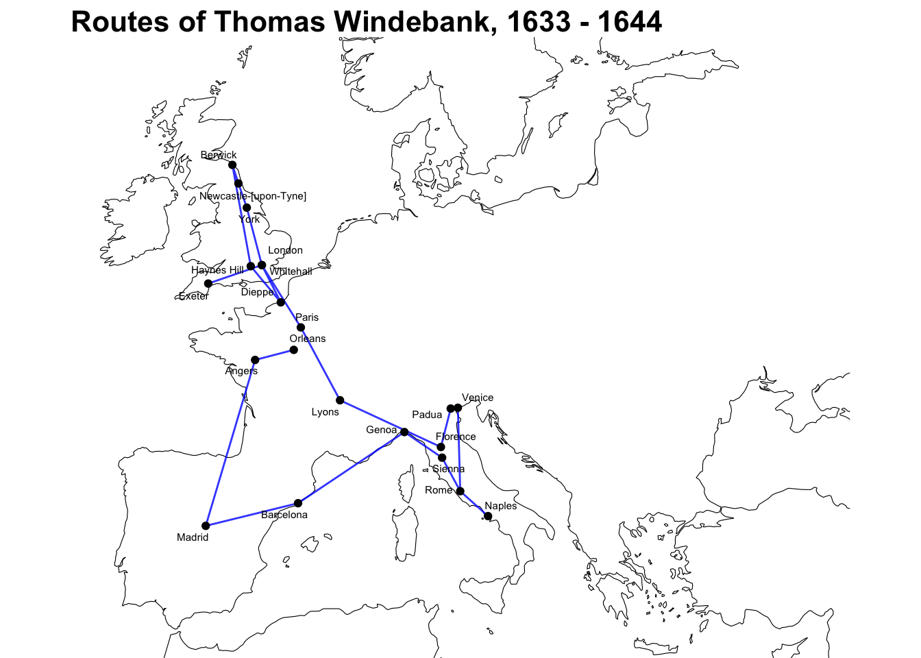
To show how these routes look like in practice, we’ll map the travels of Thomas Windebank - son of Francis Windebank, Secretary of State of Charles I. You can see by looking at his letter origins that he travelled extensively between 1633 and 1644, sending letters from France, Spain, and Italy. He often travelled with his brother Francis, and they made the journey from Rome back to London through Italy and France together, in the spring of 1637. Many letters sent from the sons to their father during this journey have made their way to the State Papers.

sp_letters %>% 
  filter(person_id ==49024)

## # A tibble: 66 x 3
##    person_id     date place_name
##        <dbl>    <dbl> <chr>     
##  1     49024 16330728 Orleans   
##  2     49024 16331204 Orleans   
##  3     49024 16331225 Orleans   
##  4     49024 16340131 Orleans   
##  5     49024 16340221 Orleans   
##  6     49024 16340326 Orleans   
##  7     49024 16340512 Orleans   
##  8     49024 16340601 Orleans   
##  9     49024 16340603 Orleans   
## 10     49024 16340730 Angers    
## # … with 56 more rows

Load the libraries rnaturalearth and rnaturalearthdata and download a map of the world using ne_coastline.

library(rnaturalearth)
library(rnaturalearthdata)

map = ne_coastline(scale = 'medium', returnclass = 'sf') 

map = map %>% st_set_crs(4326)

Draw the map, using the ggplot geom geom_sf(). This is a special geom that correctly plots sf objects to the correct type of feature. Use filter() to just plot Windebank’s route - he’s ID 49024.

library(ggsflabel)
places_points = sp_letters_with_coordinates_sf %>% filter(person_id == 49024) %>% distinct(geometry, .keep_all = T)

places_points = places_points %>% st_set_crs(4326)

p = ggplot() + 
  geom_sf(data = map, lwd = .2) + 
  geom_sf(data = lines_sf %>% 
            filter(person_id == 49024), color = 'blue', alpha = .8) + 
  geom_sf(data = places_points)+ 
  geom_sf_text_repel(data = places_points, aes(label = place_name),size = 2) + 
  theme_void() + 
  coord_sf(xlim = c(-10, 35), ylim = c(36, 60)) + 
  labs(title = 'Routes of Thomas Windebank, 1633 - 1644') + 
  theme(plot.title = element_text(face = 'bold', size = 16))
p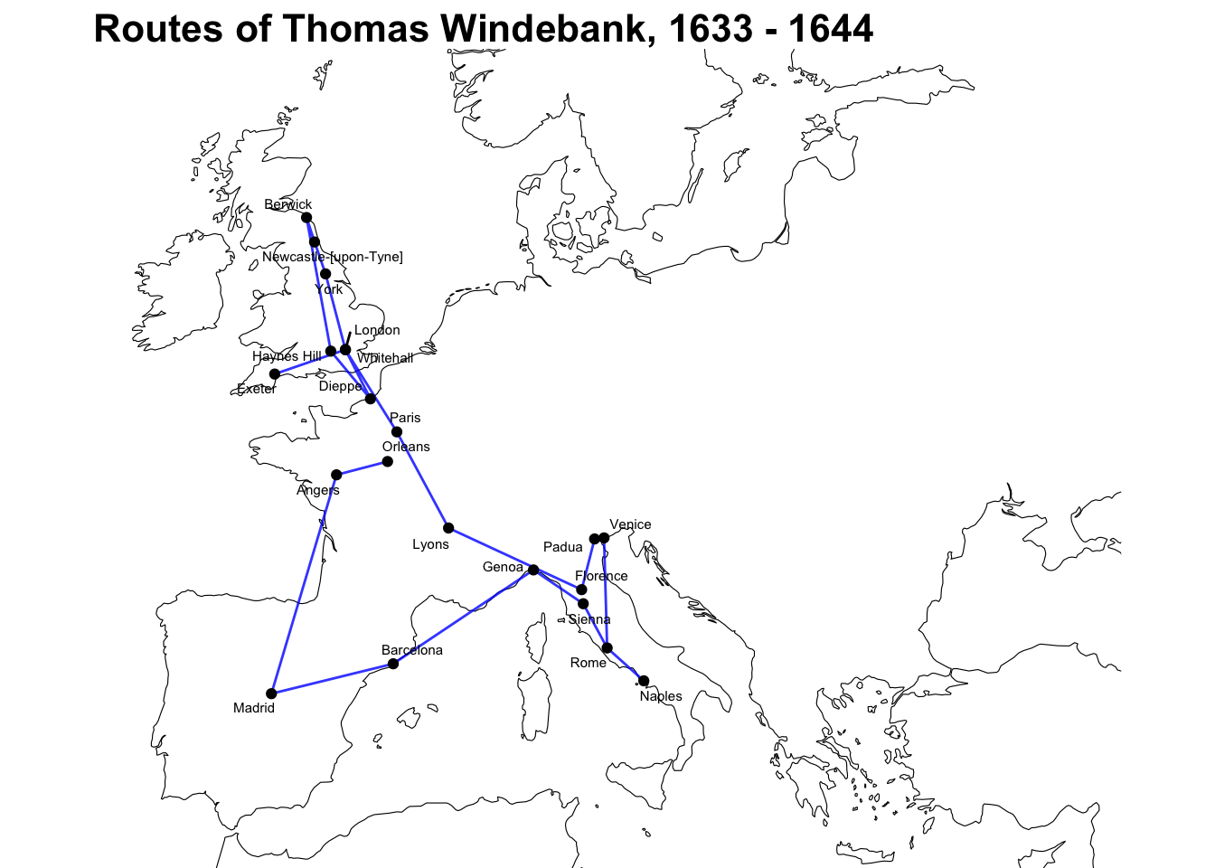

More simple features computation, using st_join()

As well as mapping and measuring lines, the simple features object can be used to perform a whole range of geo-spatial calculations and computation.

For example, one can extract all lines which pass within a given distance of a certain point.

To do this, make a simple feature object with one feature - the coordinates for Paris. I just googled the coordinates, but if you read my last blog post, you could also do this directly using Wikidata. Make sure to set the CRS.

paris = tibble(place = 'paris', coordinates_latitude = 2.352222, coordinates_longitude = 48.856613)

paris_sf = st_as_sf(paris, coords = c('coordinates_latitude' , 'coordinates_longitude'))

paris_sf = paris_sf %>% 
  st_set_crs(4326)

Next, use st_join(), a function from the sf package which performs spatial joins. Instead of joining on a key, a spatial join joins two sf datasets together using a spatial operation - which could be ‘intersects’, ‘touches’, or ‘is within distance of’, as used here.

Using st_join, join the lines_sf object (the collection of lines for each person) with the newly-created paris_sf object. We need to specify the join type (st_is_within_distance), the maximum distance, and that we only want to keep the rows where there is a successful join (i.e where the line at some point is within 100 kilometres of Paris), specified by the argument left = FALSE.

This could be useful for finding individuals who likely passed through a certain place but didn’t send a letter from there.

paris_lines = st_join(lines_sf, paris_sf, join = st_is_within_distance, dist = 100, left = FALSE) 

paris_lines

## Simple feature collection with 11 features and 3 fields
## geometry type:  LINESTRING
## dimension:      XY
## bbox:           xmin: -9.1604 ymin: 38.7452 xmax: 14.25 ymax: 55.9527
## geographic CRS: WGS 84
## # A tibble: 11 x 4
##    person_id                                            geometry  distance place
##  *     <dbl>                                    <LINESTRING [°]>       [m] <chr>
##  1      7136 (4.31 52.08, -0.1275 51.50722, 0.4105 52.2459, 4.3…  3754439… paris
##  2     10405 (-0.1275 51.50722, -0.1275 51.50722, -0.1275 51.50…   687664… paris
##  3     13045 (-0.6 51.48333, -1.1 51.443, -0.337499 51.4034, -0…  7314443… paris
##  4     18991 (2.351389 48.85694, 2.351389 48.85694, 2.351389 48…  1265118… paris
##  5     24263 (-2.65595 52.0107, -2.65595 52.0107, 2.351389 48.8…  1721473… paris
##  6     27799                (-7.7116 52.3539, 2.351389 48.85694)   810654… paris
##  7     43458 (-0.1333 51.4995, -0.1275 51.50722, -0.1275 51.507…   718841… paris
##  8     43775 (2.351389 48.85694, -8.530556 51.7075, -0.1255556 … 11790169… paris
##  9     44231 (2.351389 48.85694, -2.125 49.175, -2.125 49.175, …   999702… paris
## 10     44520 (2.351389 48.85694, -0.1275 51.50722, -0.1275 51.5…  1199219… paris
## 11     49024 (1.904167 47.90222, 1.904167 47.90222, 1.904167 47…  6506617… paris

The resulting 11 lines:

ggplot() + 
  geom_sf(data = map, lwd = .2) + 
  geom_sf(data = paris_lines) + 
  theme_void() + 
  coord_sf(xlim = c(-10, 35), ylim = c(36, 60))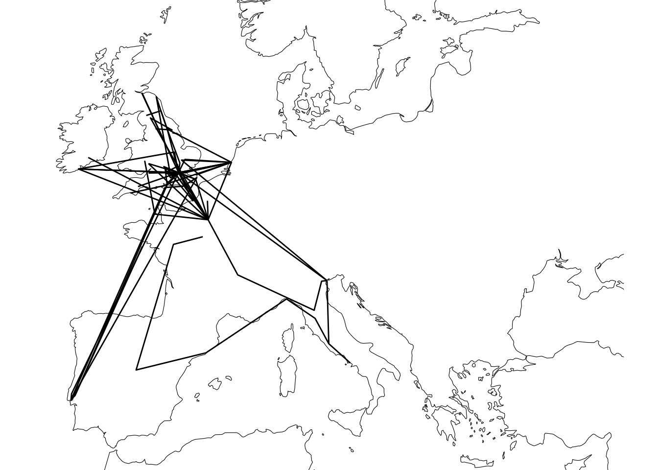

Were these lines combined with a road network as found in Campop we could plot likely paths along established routes, and then check those routes to see if they came within a certain distance of a given point.

Intersecting lines and polygons

Another join method performs a match if a line intersects a polygon. This can be used to find a list of routes which passed within a given border, a country, say.

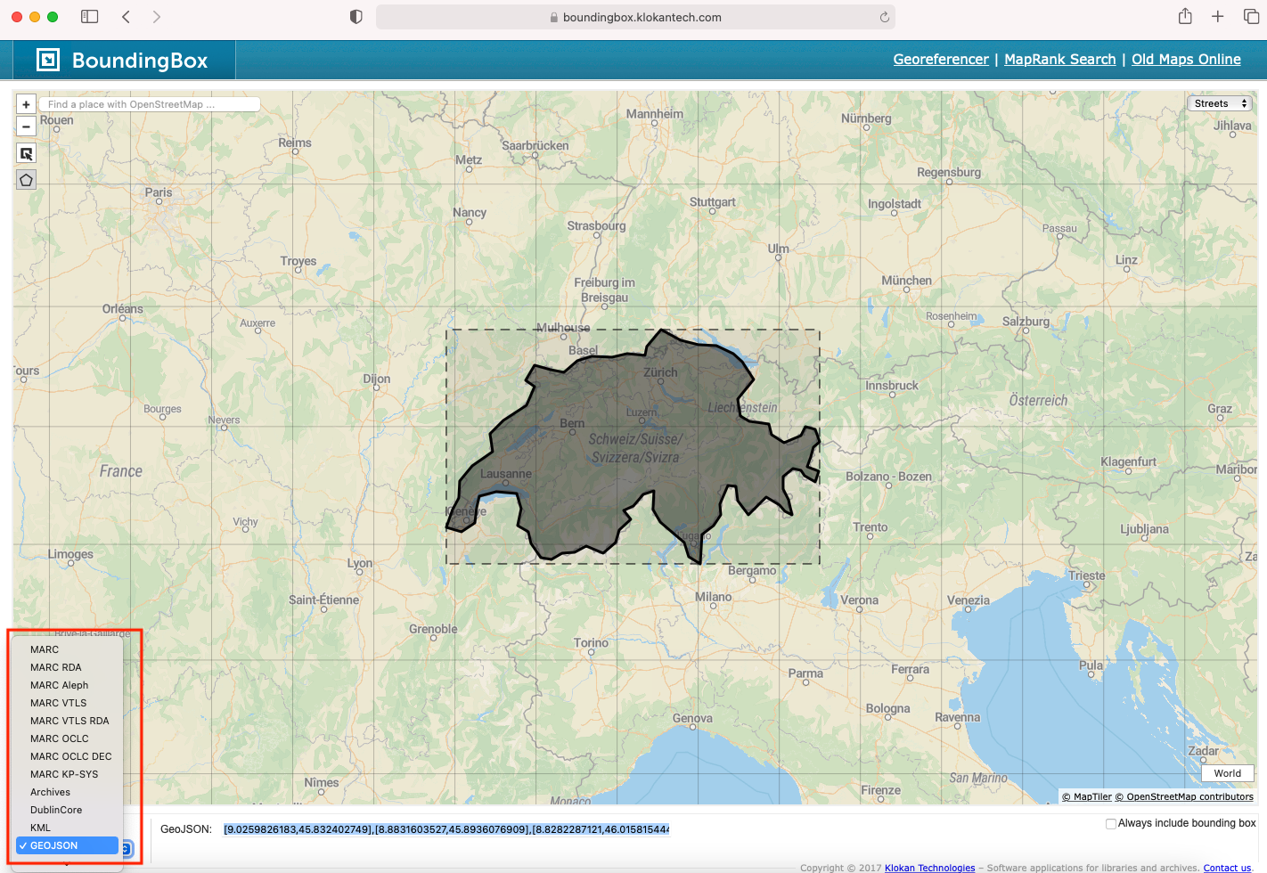
To do this, first go to (https://boundingbox.klokantech.com/) and draw a polygon around the border of modern-day Switzerland (or any other boundary you’re interested in) using the polygon tool on the top-left of the map (highlighted in red in the image below). This could also be done with a package like osm, but I like the flexibility of drawing my own border, especially for historical data.

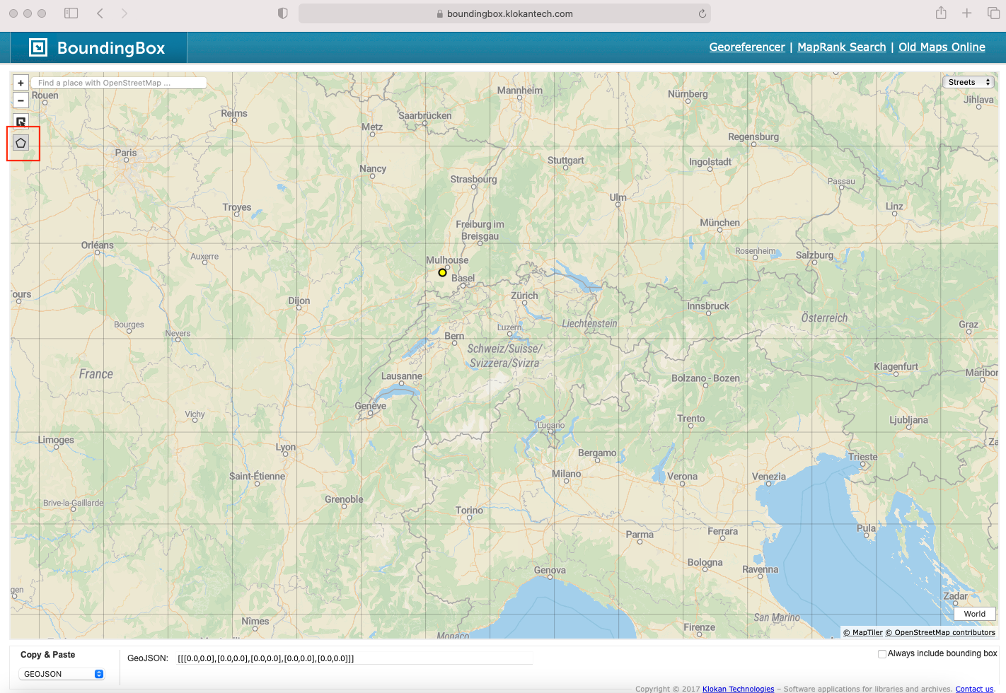
Once that’s done, use the drop-down on the bottom-left to change the format to geoJSON.

Then copy and paste the result in between the following code:

'{"type":"LineString","coordinates":[**the geoJSON result goes here***]}'

Save this as a variable called switzerland_polygon

library(geojsonsf)

switzerland_polygon <- '{"type":"LineString","coordinates":[[9.0259826183,45.832402749],[8.8831603527,45.8936076909],[8.8282287121,46.0158154441],[8.6854064465,46.0996769553],[8.5315978527,46.1910169923],[8.4437072277,46.2973888353],[8.4546935558,46.4565599202],[8.3228576183,46.4262773882],[8.202008009,46.3277429091],[8.0811583996,46.2897976864],[8.1690490246,46.213828322],[8.026226759,46.1225261729],[7.9822814465,46.0158154441],[7.8284728527,45.9241848947],[7.6197326183,45.9852887707],[7.4769103527,45.9318265638],[7.323101759,45.9241848947],[7.1912658215,45.8706637339],[7.059429884,45.8859607581],[6.9385802746,46.0081853548],[6.9056212902,46.1072944137],[6.7737853527,46.1605871525],[6.8177306652,46.3049789321],[6.7627990246,46.4338495991],[6.5101134777,46.4489908651],[6.3013732433,46.4111298103],[6.268414259,46.3125679766],[6.2464416027,46.183411111],[6.0816466808,46.1072944137],[5.8948791027,46.1453659181],[5.9717833996,46.2973888353],[6.0486876965,46.3959780242],[6.0596740246,46.539750101],[6.2134826183,46.6680664278],[6.4661681652,46.7885571342],[6.4332091808,46.9387920766],[6.5980041027,47.0511924171],[6.883648634,47.1782937099],[6.9825255871,47.3348821483],[6.8726623058,47.3869754036],[6.9825255871,47.5132734828],[7.1802794933,47.4761584717],[7.3450744152,47.4538768727],[7.5098693371,47.5503622628],[7.6856505871,47.5874248145],[7.938336134,47.5800144022],[8.1251037121,47.6096497572],[8.3448302746,47.5948341777],[8.3668029308,47.6688701199],[8.5425841808,47.8092495052],[8.7842833996,47.7206328783],[9.0040099621,47.6836647227],[9.2237365246,47.6762679456],[9.432476759,47.6096497572],[9.5423400402,47.5429466051],[9.6851623058,47.3944130985],[9.4874083996,47.2305413089],[9.520367384,47.0886066639],[9.6302306652,47.043706416],[9.871929884,47.0212421089],[9.9048888683,46.9312903141],[10.0586974621,46.863727159],[10.2674376965,46.9237875008],[10.3223693371,46.9987683457],[10.4432189465,46.9762851258],[10.4981505871,46.8712383803],[10.4212462902,46.8261552861],[10.3882873058,46.7434046605],[10.3443419933,46.6605268215],[10.487164259,46.6228130165],[10.4432189465,46.5321926165],[10.311383009,46.5850729212],[10.2674376965,46.6303578807],[10.1685607433,46.6454444542],[10.047711134,46.5775217472],[10.047711134,46.4716948745],[10.1136291027,46.38082203],[10.1575744152,46.2518261579],[10.0696837902,46.2822054852],[10.0037658215,46.335328797],[9.8389708996,46.4035544433],[9.6192443371,46.2518261579],[9.4874083996,46.3732424548],[9.4654357433,46.4943894167],[9.3665587902,46.5019521603],[9.2676818371,46.3429136328],[9.2786681652,46.2518261579],[9.1907775402,46.1605871525],[9.0479552746,46.0844388809],[9.0259826183,45.832402749]]}'

Using the function geojson_sf() convert it to an sf object, cast it to a polygon, add a column called place with the value ‘Switzerland’

switz_sf <- geojson_sf(switzerland_polygon)

switz_sf = st_as_sf(switz_sf)

switz_sf = switz_sf %>% st_cast('POLYGON')


switz_sf = switz_sf %>% st_set_crs(4326)

swiss_lines = st_join(lines_sf,switz_sf, left = FALSE)

Joining this to the sp_people dataset shows that the following routes passed through Switzerland, as the crow flies at least (as mentioned, this doesn’t work for ship captains):

swiss_lines %>% left_join(sp_people, by = 'person_id') %>% select(person_name)

## Simple feature collection with 3 features and 1 field
## geometry type:  LINESTRING
## dimension:      XY
## bbox:           xmin: -6.265833 ymin: 38.41273 xmax: 27.13838 ymax: 53.3425
## geographic CRS: WGS 84
## # A tibble: 3 x 2
##   person_name                                                           geometry
##   <chr>                                                         <LINESTRING [°]>
## 1 Captain Jonas Poole       (12.33194 45.43972, 12.33194 45.43972, 1.4897 51.18…
## 2 Dudley Carleton, Viscoun… (-0.6 51.48333, -1.1 51.443, -0.337499 51.4034, -0.…
## 3 Sir Gilbert Talbot        (12.33194 45.43972, 4.399722 51.22111, 4.35 50.85, …

A map of these routes:

ggplot() + 
  geom_sf(data = map, lwd = .2) + 
  geom_sf(data = swiss_lines) +
  geom_sf(data= switz_sf, color = 'blue', fill = NA, alpha = .7)+ 
  theme_void() + 
  coord_sf(xlim = c(-10, 35), ylim = c(36, 60))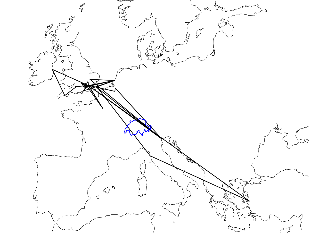

Thomas Windebank’s River Crossings

One last demonstration, showing how this spatial data can be combined with external spatial datasets to perform new operations. We’ll use the sf lines object plus a dataset of world rivers, to find a list of all major rivers Thomas Windebank had to cross during his voyages.

First, download an sf dataset of rivers from Natural Earth:

rivers50 <- ne_download(scale = 50, type = 'rivers_lake_centerlines', category = 'physical', returnclass = 'sf' )

## OGR data source with driver: ESRI Shapefile 
## Source: "/private/var/folders/17/s_d6htjx57q4x5cvv20gjthm0000gq/T/RtmpYJBHZg", layer: "ne_50m_rivers_lake_centerlines"
## with 462 features
## It has 32 fields
## Integer64 fields read as strings:  ne_id

rivers50 = rivers50 %>% st_set_crs(4326)

Returning to the route of Thomas Windebank, above, which rivers did he cross or travel near?

Use st_join() again, this time with the rivers dataset as x, and Thomas Windebank’s route as y. This will filter to show only rivers within 10,000 metres of Windebank’s route.

tw_rivers = st_join(rivers50,lines_sf %>% 
            filter(person_id == 49024),  join = st_is_within_distance, dist = 10000, left = FALSE)

Draw a map to check the results, rivers also drawn on the map, and labeled (with a weird typo in the Natural Earth dataset for the river Tagus):

ggplot() + 
  geom_sf(data = map, lwd = .2) + 
  geom_sf(data = lines_sf %>% 
            filter(person_id == 49024), alpha =.6) +
  geom_sf(data= tw_rivers, color = 'blue', fill = NA, alpha = .9)+
  geom_sf_label_repel(data= tw_rivers, alpha = .9, aes(label = name_en), size = 2.5) + 
  theme_void() + 
  coord_sf(xlim = c(-10, 35), ylim = c(36, 60)) + 
  labs(title = "Major Rivers Crossed by Thomas Windebank") + 
  theme(plot.title = element_text(size = 16, face = 'bold'))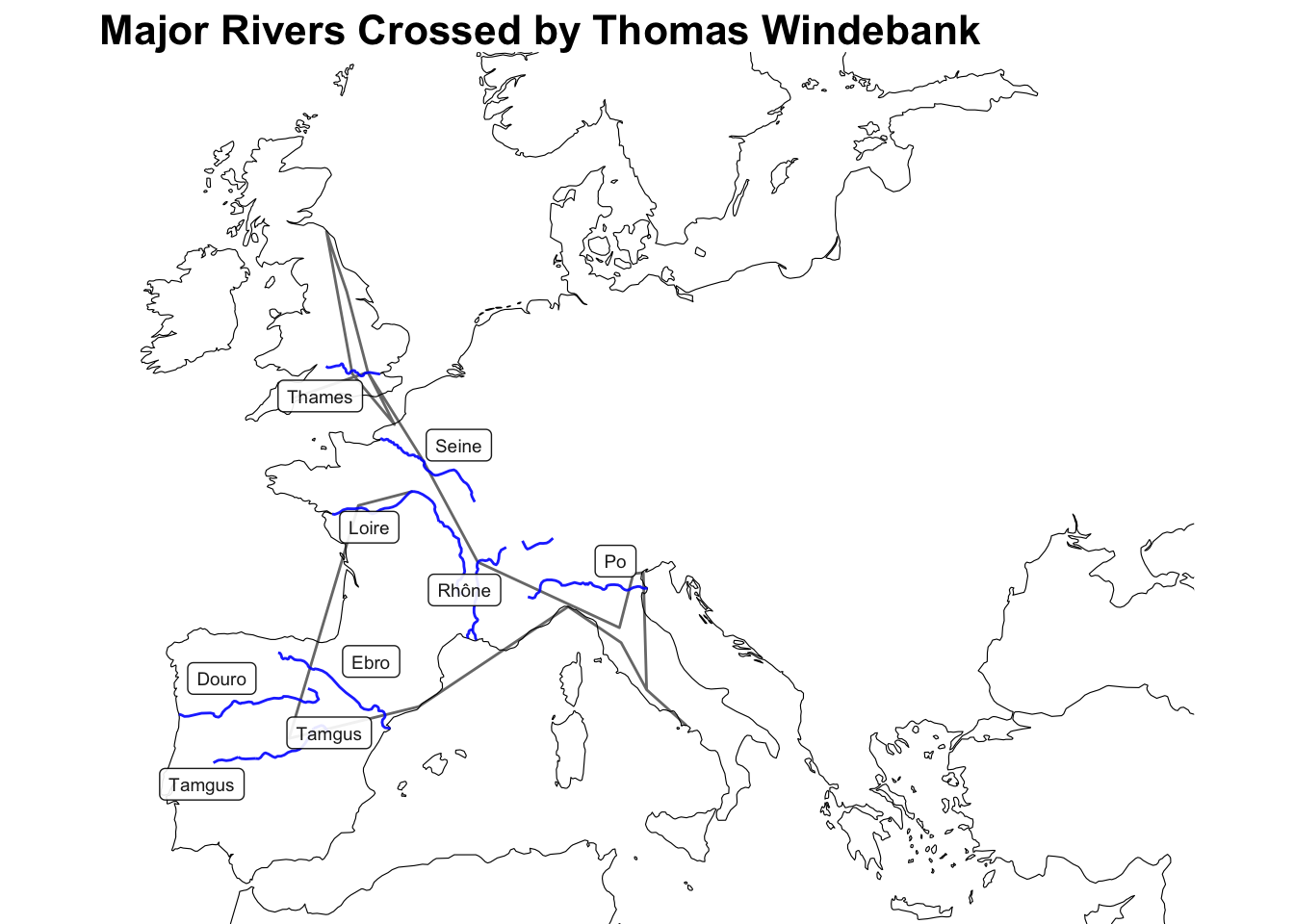

Other Uses

Representing these routes as spatial features has great potential. With a dataset of early modern roads, for example, one could calculate the likely path of each route, rather than measuring and mapping as the crow flies. Combined with date information and an average speed of movement, we could guess when an author on the road may have crossed paths with others, or if they may have been caught up in a particular event, such as a battle or siege. Wikidata even has lists of battles, complete with coordinates, which could be used as a starting point.

Special Thanks

This post is based on work by the whole Networking Archives team (past and present). A special thank-you to Miranda, who has curated and cleaned much of the State Papers geographic data - none of this would be possible without that work!