Text and Models
What can a body of text tell us about the worldview of its authors? Many Digital Humanities projects involve constructing models: a general name for a kind of representation of something which makes it in some way easier to interpret. TEI-encoded text is an example of a model: we take the ‘raw material’ of a document, its text, and add elements to it to make it easier to work with and analyse.
Models are often further abstracted from the original text. One way we can represent text in a way that a machine can interpret is with a word vector. A word vector is simply a numerical representation of a word within a corpus (a body of text, often a series of documents), usually consisting of a series of numbers in a specified sequence. This type of representation is used for a variety of Natural Language Processing tasks - for instance measuring the similarity between two documents.
This post uses a couple of R packages and a method for creating word vectors with a neural net, called GloVe, to produce a series of vectors which give useful clues as to the semantic links between words in a corpus. The method is then used to analyse the printed summaries of the English State Papers, from State Papers Online, and show how they can be used to understand how the association between words and concepts changed over the course of the seventeenth century.
What is a Word Vector, Then?
First, I’ll try to briefly explain word vectors. Imagine you have two documents in a corpus. One of them is an article about pets, and the other is a piece of fiction about a team of crime fighting animal superheroes. We’ll call them document A and document B. One way to represent the words within these documents as a vector would be to use the counts of each word per document.
To do this, you could give each word a set of coordinates, \(x\) and \(y\), where \(x\) is a count of how many times the word appears in document A and \(y\) the number of times it appears in document B.
The first step is to make a dataframe with the relevant counts:
library(ggrepel)
library(tidyverse)
word_vectors = tibble(word = c('crufts', 'feed', 'cat', 'dog', 'mouse', 'rabbit', 'cape', 'hero' ),
      x = c(10, 8, 6, 5, 6, 5, 2, 1),
      y = c(0, 1, 3, 5, 8, 8, 10, 9))

word_vectors
## # A tibble: 8 x 3
## word x y
## <chr> <dbl> <dbl>
## 1 crufts 10 0
## 2 feed 8 1
## 3 cat 6 3
## 4 dog 5 5
## 5 mouse 6 8
## 6 rabbit 5 8
## 7 cape 2 10
## 8 hero 1 9It’s likely that some words will occur mostly in document A, some mostly in document B, and some evenly spread across both. This data can be represented as a two-dimensional plot where each word is placed on the x and y axes based on their x and y values, like this:
ggplot() +
  geom_point(data = word_vectors, aes(x, y), size =4, alpha = .7) +
  geom_text_repel(data = word_vectors, aes(x, y, label = word)) +
  theme_bw() +
  labs(title = "Words Represented in Two-dimension Space") +
  theme(title = element_text(face = 'bold')) +
  scale_x_continuous(breaks = 1:10) +
  scale_y_continuous(breaks = 1:10)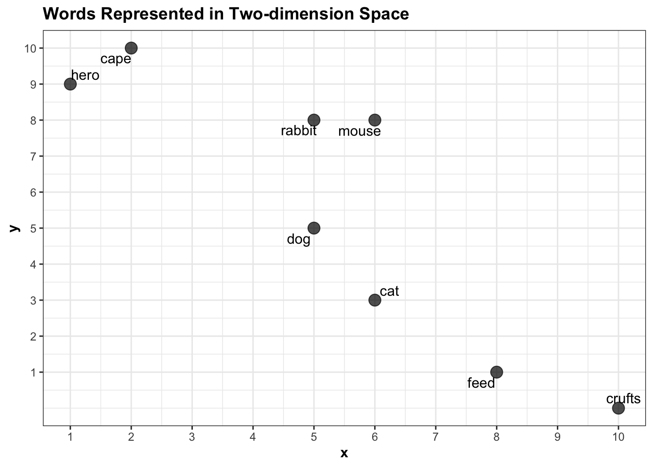
Each word is represented as a vector of length 2: ‘rabbit’ is a vector containing two numbers: {5,8}, for example. Using very basic maths we can calculate the euclidean distance between any pair of words. More or less the only thing I can remember from secondary school math is how to calculate the distance between two points on a graph, using the following formula:
\[ \sqrt {\left( {x_1 - x_2 } \right)^2 + \left( {y_1 - y_2 } \right)^2 } \]
Where \(x\) is the first point and \(y\) the second. This can easily be turned into a function in R, which takes a set of coordinates (the arguments x1 and x2) and returns the euclidean distance:
euc.dist <- function(x1, x2) sqrt(sum((pointA - pointB) ^ 2))To get the distance between ‘crufts’ and ‘mouse’, set pointA as the \(x\) and \(y\) ccoordinates for the first entry in the dataframe of coordinates we created above, and pointB the coordinates for the fifth entry:
pointA = c(word_vectors$x[1], word_vectors$y[1])
pointB = c(word_vectors$x[5], word_vectors$y[5])

euc.dist(pointA, pointB)
## [1] 8.944272Representing a pair of words as vectors and measuring the distance between them is commonly used to suggest a semantic link between the two. For instance, the distance between hero and cape in this corpus is small, because they have similar properties: they both occur mostly in the document about superheroes and rarely in the document about pets.
pointA = c(word_vectors$x[word_vectors$word == 'hero'], word_vectors$y[word_vectors$word == 'hero'])

pointB = c(word_vectors$x[word_vectors$word == 'cape'], word_vectors$y[word_vectors$word == 'cape'])

euc.dist(pointA, pointB)
## [1] 1.414214This suggests that the model has ‘learned’ that in this corpus, hero and cape are semantically more closely linked than other pairs in the dataset. The difference between cape and feed, on the other hand, is large, because one appears often in the superheroes article and rarely in the other, and vice versa.
pointA = c(word_vectors$x[word_vectors$word == 'cape'], word_vectors$y[word_vectors$word == 'cape'])

pointB = c(word_vectors$x[word_vectors$word == 'feed'], word_vectors$y[word_vectors$word == 'feed'])

euc.dist(pointA, pointB)
## [1] 10.81665Multi-Dimensional Vectors
These vectors, each consisting of two numbers, can be thought of as two-dimensional vectors: a type which can be represented on a 2D scatterplot as \(x\) and \(y\). It’s very easy to add a third dimension, \(z\):
word_vectors_3d = tibble(word = c('crufts', 'feed', 'cat', 'dog', 'mouse', 'rabbit', 'cape', 'hero' ),
      x = c(10, 8, 6, 5, 6, 5, 2, 1),
      y = c(0, 1, 3, 5, 8, 8, 10, 9),
      z = c(1,3,5,2,7,8,4,3))
Just like the plot above, we can plot the words in three dimensions, using Plotly:
library(plotly)

plot_ly(data = word_vectors_3d, x =  ~x, y = ~y,z =  ~z, text = ~word) %>% add_markers() %>% layout(title = "3D Representation of Word Vectors")
You can start to understand how the words now cluster together in the 3D plot: rabbit and mouse are still clustered together, but whereas before both were closer to dog than to cat, now it looks like they are fairly equidistant from both. We can use the same formula as above to calculate these distances, just by adding the z coordinates to the pointA and pointB vectors:
pointA = c(word_vectors_3d$x[word_vectors_3d$word == 'dog'], word_vectors_3d$y[word_vectors_3d$word == 'dog'], word_vectors_3d$z[word_vectors_3d$word == 'dog'])
pointB = c(word_vectors_3d$x[word_vectors_3d$word == 'mouse'], word_vectors_3d$y[word_vectors_3d$word == 'mouse'], word_vectors_3d$z[word_vectors_3d$word == 'mouse'])

euc.dist(pointA, pointB)
## [1] 5.91608pointA = c(word_vectors_3d$x[word_vectors_3d$word == 'cat'], word_vectors_3d$y[word_vectors_3d$word == 'cat'], word_vectors_3d$z[word_vectors_3d$word == 'cat'])
pointB = c(word_vectors_3d$x[word_vectors_3d$word == 'mouse'], word_vectors_3d$y[word_vectors_3d$word == 'mouse'], word_vectors_3d$z[word_vectors_3d$word == 'mouse'])
euc.dist(pointA, pointB)## [1] 5.385165The nice thing about the method is that while my brain starts to hurt when I think about more than three dimensions, the maths behind it doesn’t care: you can just keep plugging in longer and longer vectors and it’ll continue to calculate the distances as long as they are the same length. This means you can use this same formula not just when you have x and y coordinates, but also z, a, b, c, d, and so on for as long as you like. This is often called ‘representing words in multi-dimensional euclidean space’, or something similar which sounds great on grant applications but it’s really just doing some plotting and measuring distances. Which means that if you represent all the words in a corpus as a long vector (series of coordinates), you can quickly measure the distance between any two.
Querying the Vectors Using Arithmetic
In a large corpus with a properly-constructed vector representation, the semantic relationships between the words start to represent some sort of meaning between words and concepts in the underlying source text. It’s quite easy to perform arithmetic on vectors: you can add, subtract, divide and multiply the vectors together to get new ones, and then find the closest words to those.
Here, I’ve created a new vector, which is pointA - pointB (dog minus mouse). Then loop through each vector and calculate the distance from this vector to each word in the dataset:
pointC = pointA - pointB

df_for_results = tibble()
for(i in 1:8){

  pointA = c(word_vectors_3d$x[i], word_vectors_3d$y[i], word_vectors_3d$z[i])
  u = tibble(dist = euc.dist(pointC, pointA), word = word_vectors_3d$word[i])
  df_for_results = rbind(df_for_results, u)
}

df_for_results %>% arrange(dist)
## # A tibble: 8 x 2
## dist word
## <dbl> <chr>
## 1 0 mouse
## 2 1.41 rabbit
## 3 5.39 cat
## 4 5.39 cape
## 5 5.92 dog
## 6 6.48 hero
## 7 8.31 feed
## 8 10.8 cruftsThe closest to dog minus mouse is hero, with this vector representation. In this very tiny dataset this is meaningless, but with a large trained set, as will be shown below, it can give really interesting results.
From Vectors to Word Embeddings
These vectors are also known as word embeddings. Real algorithms base the vectors on more sophisticated metrics than that I used above. Some, such as GloVe record co-occurrence probabilities (the likelihood of every pair of words in a corpus to co-occur within a set ‘window’ of words either side), using a neural network, and pre-trained over enormous corpora of text. The resulting vectors are often used to represent the relationships between modern meanings of words, to track semantic changes over time, or to understand the history of concepts, though it’s worth pointing out they’re only as representative as the corpus used (many use sources such as Wikipedia, or Reddit, mostly produced by white men and so there’s a danger of biases towards those groups).
Word embeddings are often critiqued as reflecting or propogating bias (I highly recommend Kaspar Beelen’s post and tools to understand more about this) of their source texts. The source used here is a corpus consisting of the printed summaries of the Calendars of State Papers, which I’ve described in detail here. As such it is likely highly biased, but if the purpose of an analysis is historical, for example to understand how a concept was represented at a given time, by a specific group, in a particular body of text, the biases captured by word embeddings can be seen as a research strength rather than a weakness. The data is in no way representative of early modern text more generally, and, what’s more, the summaries were written in the 19th century and so will reflect what editors at the time thought was important. In these two ways, the corpus will reproduce a very particular wordview of a very specific group, at a very specific time. Because of this, can use the embeddings to get an idea of how certain words or ideas were semantically linked, specifically in the corpus of calendar abstracts. The data will not show us how early modern concepts were related, but it might show conceptual changes in words within the information apparatus of the state.
The following instructions are adapted from the project vignette and this tutorial. It uses the package text2vec, through which it’s possible to train the GloVe algorithm using R. First, tokenise all the abstract text and remove very common words called stop words:
library(text2vec)
library(tidytext)
library(textstem)
data("stop_words")
Next, load and pre-process the abstract text:
spo_raw = read_delim('/Users/Yann/Documents/MOST RECENT DATA/fromto_all_place_mapped_stuart_sorted', delim = '\t', col_names = F )
spo_mapped_people = read_delim('/Users/Yann/Downloads/people_docs_stuart_200421', delim = '\t', col_names = F)

load('/Users/Yann/Documents/non-Github/spo_data/g')
g = g %>% group_by(path) %>% summarise(value = paste0(value, collapse = "<br>"))

spo_raw = spo_raw %>%
mutate(X7 = str_replace(X7, "spo", "SPO")) %>%
separate(X7, into = c('Y1', 'Y2', 'Y3'), sep = '/') %>%
mutate(fullpath = paste0("/Users/Yann/Documents/non-Github/spo_xml/", Y1, '/XML/', Y2,"/", Y3)) %>% mutate(uniquecode = paste0("Z", 1:nrow(spo_raw), "Z"))

withtext = left_join(spo_raw, g, by = c('fullpath' = 'path')) %>%
left_join(spo_mapped_people %>% dplyr::select(X1, from_name = X2), by = c('X1' = 'X1'))%>%
left_join(spo_mapped_people %>% dplyr::select(X1, to_name = X2), by = c('X2' = 'X1'))
Tokenize the text using the function unnest_tokens() from the Tidytext library, remove stop words, lemmatize the text (reduce the words to their stem) using textstem, and filter out any words which are actually just numbers. unnest_tokens makes a new dataframe based on the inputted text, with one word per row, which can then be counted, sorted, filtered and so forth.
words = withtext %>%
  ungroup()  %>%
  select(document = X5, value, date = X3) %>%
  unnest_tokens(word, value) %>% anti_join(stop_words)%>%
  mutate(word = lemmatize_words(word)) %>% filter(!str_detect(word, "[0-9]{1,}"))
Create a ‘vocabulary’ with the word2vec package, which is just a list of each word found in the dataset and the times they occur, and ‘prune’ it to only words which occur at least five times.
words_ls = list(words$word)

it = itoken(words_ls, progressbar = FALSE)

vocab = create_vocabulary(it)

vocab = prune_vocabulary(vocab, term_count_min = 5)
With the vocabulary, next construct a ‘term co-occurence matrix’: this is a matrix of rows and columns, counting all the times each word co-occurs with every other word, within a window which can be set with the argument skip_grams_window =
vectorizer = vocab_vectorizer(vocab)

# use window of 10 for context words
tcm = create_tcm(it, vectorizer, skip_grams_window = 10)
Now use the GloVe algorithm to train the model and produce the vectors, with a set number of iterations: here we’ve used 20, which seems to give good results. It can be quite slow, but as it’s a relatively small dataset (in comparison to something like the entire English wikipedia), it shouldn’t take too long to run - a couple of minutes for 20 iterations.
glove = GlobalVectors$new(rank = 100, x_max = 10)

wv_main = glove$fit_transform(tcm, n_iter = 20, convergence_tol = 0.00001)
## INFO [14:33:52.149] epoch 1, loss 0.1507
## INFO [14:34:14.703] epoch 2, loss 0.0991
## INFO [14:34:37.552] epoch 3, loss 0.0877
## INFO [14:35:00.521] epoch 4, loss 0.0816
## INFO [14:35:23.633] epoch 5, loss 0.0777
## INFO [14:35:46.241] epoch 6, loss 0.0749
## INFO [14:36:09.263] epoch 7, loss 0.0727
## INFO [14:36:32.052] epoch 8, loss 0.0710
## INFO [14:36:54.664] epoch 9, loss 0.0696
## INFO [14:37:17.249] epoch 10, loss 0.0684
## INFO [14:37:39.803] epoch 11, loss 0.0674
## INFO [14:38:02.554] epoch 12, loss 0.0666
## INFO [14:38:25.339] epoch 13, loss 0.0658
## INFO [14:38:48.060] epoch 14, loss 0.0652
## INFO [14:39:10.665] epoch 15, loss 0.0646
## INFO [14:39:33.385] epoch 16, loss 0.0641
## INFO [14:39:56.206] epoch 17, loss 0.0636
## INFO [14:40:19.104] epoch 18, loss 0.0632
## INFO [14:40:41.794] epoch 19, loss 0.0628
## INFO [14:41:04.779] epoch 20, loss 0.0625GloVe results in two sets of word vectors. The authors of the GloVe package suggest that combining both results in higher-quality embeddings:
wv_context = glove$components


# Either word-vectors matrices could work, but the developers of the technique
# suggest the sum/mean may work better
word_vectors = wv_main + t(wv_context)
Results
The next step was to write a small function which calculates and displays the closest words to a given word, to make it easier to query the results. There’s an important change here: instead of using the euclidean distance formula above, distance is calculated using the cosine similarity, which measures the angular distance between the words (this is better because it corrects for one word appearing many times and another appearing very infrequently).
ten_closest_words = function(word){

word_result = word_vectors[word, , drop = FALSE]

cos_sim = sim2(x = word_vectors, y = word_result, method = "cosine", norm = "l2")


head(sort(cos_sim[,1], decreasing = TRUE), 20)

}
The function takes a single word as an argument and returns the twenty closest word vectors, by cosine distance. What are the closest in useage to king?
ten_closest_words('king')## king king's majesty queen majesty's prince england declare
## 1.0000000 0.8177222 0.8105912 0.7352217 0.7151208 0.7126855 0.7119099 0.7046366
## seq late duke please lord promise cpg grant
## 0.7032410 0.7006746 0.7004456 0.7000613 0.6895407 0.6870112 0.6819107 0.6768820
## intend id pray favour
## 0.6747779 0.6738966 0.6726993 0.6707538Unsurprisingly, a word that is often interchangeable with King, Majesty, is the closest, followed by Queen - also obviously interchangeable with King, depending on the circumstances.
Word embeddings are often used to understand different and changing gender representations. How are gendered words represented in the State Papers abstracts? First of all, wife:
ten_closest_words('wife')## wife husband child sister mother lady brother daughter
## 1.0000000 0.8135368 0.7680603 0.7517228 0.7248175 0.7231804 0.7188545 0.7139700
## marry father widow son family servant life live
## 0.6806173 0.6671037 0.6567243 0.6479807 0.6139687 0.6107722 0.6105448 0.6018107
## friend writer's woman die
## 0.5981722 0.5951051 0.5904939 0.5851097It seems that wife is most similar to other words relating to family. What about husband?
ten_closest_words('husband')## husband wife child widow lady sister
## 1.0000000 0.8135368 0.7335813 0.6727104 0.6109208 0.6007251
## mother brother daughter servant husband's son
## 0.5964263 0.5954335 0.5932350 0.5907590 0.5786800 0.5739544
## marry woman father die debt family
## 0.5711938 0.5702857 0.5698491 0.5679301 0.5675128 0.5576354
## petition petitioner's
## 0.5541463 0.5466416Husband is mostly similar but with some interesting different associations: widow, die, petition, debt, and prisoner, reflecting the fact that there is a large group of petitions in the State Papers written by women looking for pardons or clemency for their husbands, particularly following the Monmouth Rebellion in 1683.
Looking at the closest words to place names gives some interesting associations. Amsterdam is associated with terms related to shipping and trade:
ten_closest_words('amsterdam')## amsterdam rotterdam lade bordeaux hamburg richly
## 1.0000000 0.7889888 0.6468717 0.6042075 0.5822187 0.5647650
## holland zealand dutch prize merchant vessel
## 0.5594555 0.5447143 0.5356518 0.5309154 0.5261446 0.5255347
## arrive flush ostend ship london copenhagen
## 0.5245304 0.5159787 0.5138438 0.5103055 0.5003312 0.4997833
## merchantmen cadiz
## 0.4943865 0.4898490Whereas Rome is very much associated with religion and ecclesiastical politics:
ten_closest_words('rome')## rome pope jesuit friar priest naples catholic
## 1.0000000 0.6087960 0.5907551 0.5596762 0.5415235 0.5409374 0.5321532
## spain venice cardinal nuncio germany italy pope's
## 0.5181883 0.5172574 0.5070520 0.4870522 0.4813966 0.4804191 0.4593149
## religion paris ambassador tyrone florence archdukes
## 0.4531869 0.4531597 0.4467086 0.4433518 0.4343476 0.4239177More Complex Vector Tasks
As well as finding the most similar words, we can also perform arithmetic on the vectors. What are the closest words to book plus news?
sum = word_vectors["book", , drop = F] +
 word_vectors["news", , drop = F]

cos_sim_test = sim2(x = word_vectors, y = sum, method = "cosine", norm = "l2")

head(sort(cos_sim_test[,1], decreasing = T), 20)
## news book letter send account hear enclose
## 0.8022483 0.8007200 0.7002376 0.6938228 0.6865210 0.6698032 0.6659100
## return write print day hope williamson post
## 0.6578209 0.6575487 0.6477301 0.6463922 0.6396193 0.6342159 0.6332963
## bring expect hand receive report note
## 0.6306521 0.6289672 0.6241833 0.6197365 0.6183798 0.6177360This is a way of finding semantically-linked analogies beyond simply two equivalent words. So, for example, Paris - France + Germany should equal to Berlin, because Berlin is like the Paris of France. It’s the equivalent of those primary school exercises ‘Paris is to France as ____ is to Germany’. As the word vectors are numbers, they can be added and subtracted. What does the State Papers corpus think is the Paris of Germany?
test = word_vectors["paris", , drop = F] -
  word_vectors["france", , drop = F] +
  word_vectors["germany", , drop = F]

#+
 # shakes_word_vectors["letter", , drop = F]

cos_sim_test = sim2(x = word_vectors, y = test, method = "cosine", norm = "l2")

head(sort(cos_sim_test[,1], decreasing = T), 10)
## germany paris brussels ps advertisement
## 0.6135925 0.5852843 0.5315038 0.4704347 0.4452859
## frankfort hague edmonds n.s curtius
## 0.4311039 0.4200639 0.4137443 0.4008544 0.4005619After Germany and Paris, the most similar to Paris - France + Germany is Brussels: not the correct answer, but a close enough guess!
We can try other analogies: pen - letter + book (pen is to letter as _____ is to book) should in theory give some word related to printing and book production such as print, or press, or maybe type:
test = word_vectors["pen", , drop = F] -
  word_vectors["letter", , drop = F] +
    word_vectors["book", , drop = F]

cos_sim_test = sim2(x = word_vectors, y = test, method = "cosine", norm = "l2")

head(sort(cos_sim_test[,1], decreasing = T), 20)
## pen book storekeeper's unlicensed bywater's
## 0.5719533 0.5393821 0.5175164 0.4966075 0.4912080
## pamphlet ink pareus waterton aloft
## 0.4897688 0.4665493 0.4471487 0.4383422 0.4297689
## schismatical stitch catalogue humphrey's writing
## 0.4283230 0.4281081 0.4275299 0.4270771 0.4262785
## promiscuously quires closet crucifix sheet
## 0.4225891 0.4177962 0.4156617 0.4143025 0.4137616Not bad - printer is in the top 20! The closest is ink, plus some other book-production-related words like stitch, ream, and pamphlet. Though some of these words can also be associated with manuscript production, we could be generous and say that they are sort of to a book as a pen is to a letter!
Change in Semantic Relations Over Time
Another, potentially more interesting way to use a longitudinal corpus like this is to look for change in semantic meaning over time. This can be done by splitting the data into temporally distinct sections, and comparing word associations across them.
First, divide the text into four separate sections, one for each reign:
library(lubridate)
james_i = withtext %>%
  mutate(year = year(ymd(X4))) %>%
  filter(year %in% 1603:1624) %>%
  ungroup()  %>%
  select(document = X5, value, date = X3) %>%
  unnest_tokens(word, value) %>%
  anti_join(stop_words) %>%
  mutate(word = lemmatize_words(word)) %>% filter(!str_detect(word, "[0-9]{1,}"))

charles_i = withtext %>%
  mutate(year = year(ymd(X4))) %>%
  filter(year %in% 1625:1648) %>%
  ungroup()  %>%
  select(document = X5, value, date = X3) %>%
  unnest_tokens(word, value) %>% anti_join(stop_words)%>%
  mutate(word = lemmatize_words(word)) %>% filter(!str_detect(word, "[0-9]{1,}"))

commonwealth = withtext %>%
  mutate(year = year(ymd(X4))) %>%
  filter(year %in% 1649:1659) %>%
  ungroup()  %>%
  select(document = X5, value, date = X3) %>%
  unnest_tokens(word, value) %>% anti_join(stop_words)%>%
  mutate(word = lemmatize_words(word)) %>% filter(!str_detect(word, "[0-9]{1,}"))

charles_ii = withtext %>%
  mutate(year = year(ymd(X4))) %>%
  filter(year %in% 1660:1684) %>%
  ungroup()  %>%
  select(document = X5, value, date = X3) %>%
  unnest_tokens(word, value) %>% anti_join(stop_words)%>%
  mutate(word = lemmatize_words(word)) %>% filter(!str_detect(word, "[0-9]{1,}"))

james_ii_w_m_ann = withtext %>%
  mutate(year = year(ymd(X4))) %>%
  filter(year %in% 1685:1714) %>%
  ungroup()  %>%
  select(document = X5, value, date = X3) %>%
  unnest_tokens(word, value) %>% anti_join(stop_words) %>%
  mutate(word = lemmatize_words(word)) %>% filter(!str_detect(word, "[0-9]{1,}"))
Now run the same scripts as above, on each of these sections:
james_i_words_ls = list(james_i$word)
it = itoken(james_i_words_ls, progressbar = FALSE)
james_i_vocab = create_vocabulary(it)
james_i_vocab = prune_vocabulary(james_i_vocab, term_count_min = 5)

vectorizer = vocab_vectorizer(james_i_vocab)

# use window of 10 for context words
james_i_tcm = create_tcm(it, vectorizer, skip_grams_window = 10)

james_i_glove = GlobalVectors$new(rank = 100, x_max = 10)

james_i_wv_main = james_i_glove$fit_transform(james_i_tcm, n_iter = 20, convergence_tol = 0.00001)
## INFO [14:41:43.864] epoch 1, loss 0.1523
## INFO [14:41:49.539] epoch 2, loss 0.0919
## INFO [14:41:55.057] epoch 3, loss 0.0783
## INFO [14:42:00.637] epoch 4, loss 0.0711
## INFO [14:42:06.157] epoch 5, loss 0.0664
## INFO [14:42:11.731] epoch 6, loss 0.0630
## INFO [14:42:17.411] epoch 7, loss 0.0603
## INFO [14:42:23.078] epoch 8, loss 0.0582
## INFO [14:42:28.986] epoch 9, loss 0.0565
## INFO [14:42:34.595] epoch 10, loss 0.0551
## INFO [14:42:40.130] epoch 11, loss 0.0539
## INFO [14:42:45.749] epoch 12, loss 0.0528
## INFO [14:42:51.318] epoch 13, loss 0.0519
## INFO [14:42:56.928] epoch 14, loss 0.0511
## INFO [14:43:02.448] epoch 15, loss 0.0504
## INFO [14:43:07.986] epoch 16, loss 0.0498
## INFO [14:43:13.553] epoch 17, loss 0.0492
## INFO [14:43:19.060] epoch 18, loss 0.0487
## INFO [14:43:24.607] epoch 19, loss 0.0482
## INFO [14:43:30.206] epoch 20, loss 0.0478james_i_wv_context = james_i_glove$components
james_i_word_vectors = james_i_wv_main + t(james_i_wv_context)charles_i_words_ls = list(charles_i$word)
it = itoken(charles_i_words_ls, progressbar = FALSE)
charles_i_vocab = create_vocabulary(it)
charles_i_vocab = prune_vocabulary(charles_i_vocab, term_count_min = 5)
vectorizer = vocab_vectorizer(charles_i_vocab)
# use window of 10 for context words
charles_i_tcm = create_tcm(it, vectorizer, skip_grams_window = 10)
charles_i_glove = GlobalVectors$new(rank = 100, x_max = 10)
charles_i_wv_main = charles_i_glove$fit_transform(charles_i_tcm, n_iter = 20, convergence_tol = 0.00001)## INFO [14:43:53.928] epoch 1, loss 0.1505
## INFO [14:44:00.855] epoch 2, loss 0.0916
## INFO [14:44:07.849] epoch 3, loss 0.0789
## INFO [14:44:14.816] epoch 4, loss 0.0721
## INFO [14:44:21.726] epoch 5, loss 0.0676
## INFO [14:44:28.652] epoch 6, loss 0.0644
## INFO [14:44:35.547] epoch 7, loss 0.0619
## INFO [14:44:42.426] epoch 8, loss 0.0599
## INFO [14:44:49.358] epoch 9, loss 0.0582
## INFO [14:44:56.229] epoch 10, loss 0.0568
## INFO [14:45:03.211] epoch 11, loss 0.0557
## INFO [14:45:10.157] epoch 12, loss 0.0547
## INFO [14:45:17.075] epoch 13, loss 0.0538
## INFO [14:45:23.994] epoch 14, loss 0.0530
## INFO [14:45:30.845] epoch 15, loss 0.0524
## INFO [14:45:37.754] epoch 16, loss 0.0518
## INFO [14:45:44.649] epoch 17, loss 0.0512
## INFO [14:45:51.568] epoch 18, loss 0.0507
## INFO [14:45:58.520] epoch 19, loss 0.0502
## INFO [14:46:05.504] epoch 20, loss 0.0498charles_i_wv_context = charles_i_glove$components
charles_i_word_vectors = charles_i_wv_main + t(charles_i_wv_context)commonwealth_words_ls = list(commonwealth$word)
it = itoken(commonwealth_words_ls, progressbar = FALSE)
commonwealth_vocab = create_vocabulary(it)
commonwealth_vocab = prune_vocabulary(commonwealth_vocab, term_count_min = 5)
vectorizer = vocab_vectorizer(commonwealth_vocab)
# use window of 10 for context words
commonwealth_tcm = create_tcm(it, vectorizer, skip_grams_window = 10)
commonwealth_glove = GlobalVectors$new(rank = 100, x_max = 10)
commonwealth_wv_main = commonwealth_glove$fit_transform(commonwealth_tcm, n_iter = 20, convergence_tol = 0.00001)## INFO [14:46:22.417] epoch 1, loss 0.1695
## INFO [14:46:25.367] epoch 2, loss 0.0946
## INFO [14:46:28.308] epoch 3, loss 0.0789
## INFO [14:46:31.251] epoch 4, loss 0.0708
## INFO [14:46:34.185] epoch 5, loss 0.0655
## INFO [14:46:37.125] epoch 6, loss 0.0617
## INFO [14:46:40.063] epoch 7, loss 0.0587
## INFO [14:46:43.000] epoch 8, loss 0.0563
## INFO [14:46:45.933] epoch 9, loss 0.0544
## INFO [14:46:48.866] epoch 10, loss 0.0527
## INFO [14:46:51.823] epoch 11, loss 0.0513
## INFO [14:46:54.845] epoch 12, loss 0.0501
## INFO [14:46:57.898] epoch 13, loss 0.0491
## INFO [14:47:00.936] epoch 14, loss 0.0482
## INFO [14:47:03.940] epoch 15, loss 0.0474
## INFO [14:47:07.453] epoch 16, loss 0.0466
## INFO [14:47:10.495] epoch 17, loss 0.0460
## INFO [14:47:13.543] epoch 18, loss 0.0454
## INFO [14:47:16.539] epoch 19, loss 0.0448
## INFO [14:47:19.550] epoch 20, loss 0.0443commonwealth_wv_context = commonwealth_glove$components
# dim(shakes_wv_context)
# Either word-vectors matrices could work, but the developers of the technique
# suggest the sum/mean may work better
commonwealth_word_vectors = commonwealth_wv_main + t(commonwealth_wv_context)charles_ii_words_ls = list(charles_ii$word)
it = itoken(charles_ii_words_ls, progressbar = FALSE)
charles_ii_vocab = create_vocabulary(it)
charles_ii_vocab = prune_vocabulary(charles_ii_vocab, term_count_min = 5)
vectorizer = vocab_vectorizer(charles_ii_vocab)
# use window of 10 for context words
charles_ii_tcm = create_tcm(it, vectorizer, skip_grams_window = 10)
charles_ii_glove = GlobalVectors$new(rank = 100, x_max = 10)
charles_ii_wv_main = charles_ii_glove$fit_transform(charles_ii_tcm, n_iter = 20, convergence_tol = 0.00001)## INFO [14:47:49.796] epoch 1, loss 0.1464
## INFO [14:48:00.251] epoch 2, loss 0.0904
## INFO [14:48:10.819] epoch 3, loss 0.0786
## INFO [14:48:21.365] epoch 4, loss 0.0724
## INFO [14:48:31.924] epoch 5, loss 0.0684
## INFO [14:48:42.493] epoch 6, loss 0.0655
## INFO [14:48:52.952] epoch 7, loss 0.0633
## INFO [14:49:03.813] epoch 8, loss 0.0615
## INFO [14:49:14.387] epoch 9, loss 0.0601
## INFO [14:49:25.185] epoch 10, loss 0.0589
## INFO [14:49:36.102] epoch 11, loss 0.0579
## INFO [14:49:47.181] epoch 12, loss 0.0570
## INFO [14:49:57.817] epoch 13, loss 0.0562
## INFO [14:50:08.585] epoch 14, loss 0.0555
## INFO [14:50:18.848] epoch 15, loss 0.0549
## INFO [14:50:29.110] epoch 16, loss 0.0544
## INFO [14:50:39.406] epoch 17, loss 0.0539
## INFO [14:50:49.701] epoch 18, loss 0.0535
## INFO [14:51:00.145] epoch 19, loss 0.0531
## INFO [14:51:10.411] epoch 20, loss 0.0527charles_ii_wv_context = charles_ii_glove$components
# dim(shakes_wv_context)
# Either word-vectors matrices could work, but the developers of the technique
# suggest the sum/mean may work better
charles_ii_word_vectors = charles_ii_wv_main + t(charles_ii_wv_context)james_ii_w_m_ann_words_ls = list(james_ii_w_m_ann$word)
it = itoken(james_ii_w_m_ann_words_ls, progressbar = FALSE)
james_ii_w_m_ann_vocab = create_vocabulary(it)
james_ii_w_m_ann_vocab = prune_vocabulary(james_ii_w_m_ann_vocab, term_count_min = 5)
vectorizer = vocab_vectorizer(james_ii_w_m_ann_vocab)
# use window of 10 for context words
james_ii_w_m_ann_tcm = create_tcm(it, vectorizer, skip_grams_window = 10)
james_ii_w_m_ann_glove = GlobalVectors$new(rank = 100, x_max = 10)
james_ii_w_m_ann_wv_main = james_ii_w_m_ann_glove$fit_transform(james_ii_w_m_ann_tcm, n_iter = 20, convergence_tol = 0.00001)## INFO [14:51:35.394] epoch 1, loss 0.1594
## INFO [14:51:39.937] epoch 2, loss 0.0926
## INFO [14:51:44.553] epoch 3, loss 0.0788
## INFO [14:51:49.111] epoch 4, loss 0.0714
## INFO [14:51:53.655] epoch 5, loss 0.0665
## INFO [14:51:58.203] epoch 6, loss 0.0629
## INFO [14:52:02.820] epoch 7, loss 0.0601
## INFO [14:52:07.513] epoch 8, loss 0.0579
## INFO [14:52:12.080] epoch 9, loss 0.0561
## INFO [14:52:16.643] epoch 10, loss 0.0546
## INFO [14:52:21.239] epoch 11, loss 0.0533
## INFO [14:52:25.989] epoch 12, loss 0.0522
## INFO [14:52:30.580] epoch 13, loss 0.0512
## INFO [14:52:35.115] epoch 14, loss 0.0504
## INFO [14:52:39.664] epoch 15, loss 0.0496
## INFO [14:52:44.202] epoch 16, loss 0.0489
## INFO [14:52:48.739] epoch 17, loss 0.0483
## INFO [14:52:53.280] epoch 18, loss 0.0478
## INFO [14:52:57.868] epoch 19, loss 0.0472
## INFO [14:53:02.430] epoch 20, loss 0.0468james_ii_w_m_ann_wv_context = james_ii_w_m_ann_glove$components
# dim(shakes_wv_context)
# Either word-vectors matrices could work, but the developers of the technique
# suggest the sum/mean may work better
james_ii_w_m_ann_word_vectors = james_ii_w_m_ann_wv_main + t(james_ii_w_m_ann_wv_context)Write a function to query the results as we did above, this time with two arguments, so we can specify both the word and the relevant reign:
top_ten_function = function(word, period){


  if(period == 'james_i'){

  vectors = james_i_word_vectors[word, , drop = FALSE]
  cos_sim = sim2(x = james_i_word_vectors, y = vectors, method = "cosine", norm = "l2")


}
  else if(period == 'charles_i'){  vectors = charles_i_word_vectors[word, , drop = FALSE]
  cos_sim = sim2(x = charles_i_word_vectors, y = vectors, method = "cosine", norm = "l2")

  }
  else if(period == 'commonwealth')  {

    vectors = commonwealth_word_vectors[word, , drop = FALSE]
  cos_sim = sim2(x = commonwealth_word_vectors, y = vectors, method = "cosine", norm = "l2")

  }

  else if(period == 'charles_ii'){

    vectors = charles_ii_word_vectors[word, , drop = FALSE]
  cos_sim = sim2(x = charles_ii_word_vectors, y = vectors, method = "cosine", norm = "l2")

  }

  else {

  vectors = james_ii_w_m_ann_word_vectors[word, , drop = FALSE]
  cos_sim = sim2(x = james_ii_w_m_ann_word_vectors, y = vectors, method = "cosine", norm = "l2")
  }

head(sort(cos_sim[,1], decreasing = TRUE), 20)


}
We could now use this function to check individual word associations in a specfied time period. It is more useful to write a second function, which takes a word as an argument and returns a chart of the ten closest words for each reign, making them much easier to instantly compare.
first_in_each= function(word) {

  rbind(top_ten_function(word, 'james_i') %>% tibble::enframe() %>% arrange(desc(value)) %>% slice(2:11) %>% mutate(reign ='james_i' ),
     top_ten_function(word, 'charles_i') %>% tibble::enframe() %>% arrange(desc(value)) %>% slice(2:11) %>% mutate(reign ='charles_i' ),
     top_ten_function(word, 'commonwealth') %>% tibble::enframe() %>% arrange(desc(value)) %>% slice(2:11) %>% mutate(reign ='commonwealth' ),
     top_ten_function(word, 'charles_ii') %>% tibble::enframe() %>% arrange(desc(value)) %>% slice(2:11) %>% mutate(reign ='charles_ii' ),
     top_ten_function(word, 'james_ii_w_m_ann') %>% tibble::enframe() %>% arrange(desc(value)) %>% slice(2:11) %>% mutate(reign ='james_ii_w_m_ann' ))%>%
  group_by(reign) %>%
  mutate(rank = rank(value)) %>%
  ggplot() +
  geom_text(aes(x = factor(reign, levels = c('james_i', 'charles_i', 'commonwealth', 'charles_ii', 'james_ii', 'james_ii_w_m_ann')), y = rank, label = name, color = name)) +
    theme_void() +
  theme(legend.position = 'none',
        axis.text.x = element_text(face = 'bold'),
        title = element_text(face = 'bold')
        ) +
    labs(title = paste0("Ten closest semantically-linked words to '", word,"'", subtitle =  "for five periods of the 17th Century"))

  }
This can show us the changing associations of particular words over time. I’m going to give one interesting example, match.
first_in_each('match') 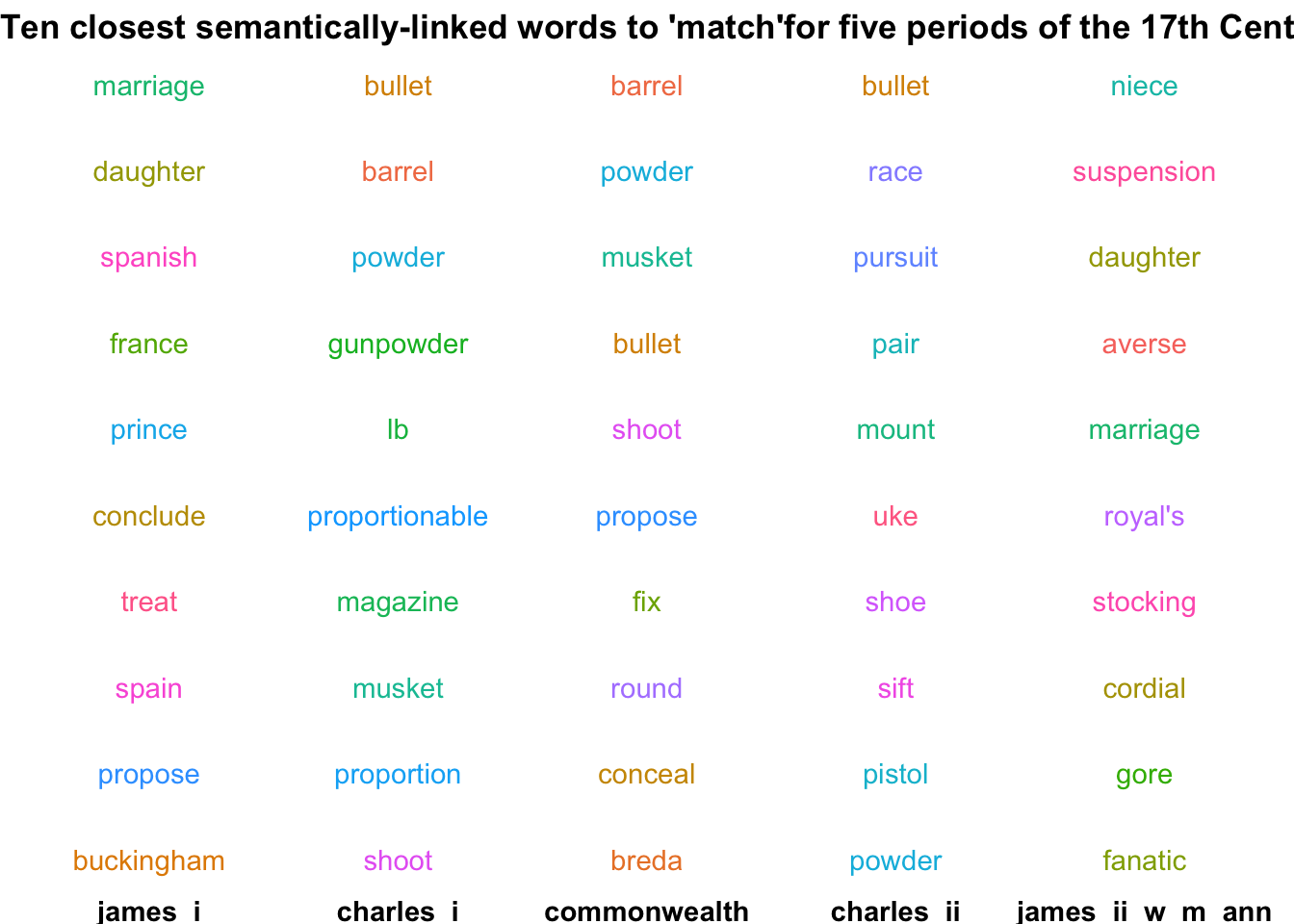
In the reign of James I, ‘match’ is semantically linked to words relating to the marriage: this is because of correspondence relating to the Spanish Match: a proposed match between Charles I and the Infanta Maria Anna of Spain, which eventually fell through. However during Charles I’s reign and afterwards, the meaning changes completely - now the closest words are all to do with the military - match here is mostly being used to refer to a component of a gun or cannon. In the final section of the data, the semantic link returns again to mostly words about marriage - this time it’s not so obvious why the words are associated, but it’s probably relating to the marriage of Philippe II, Duke of Orléans to Françoise Marie de Bourbon, in 1692 - Philippe II was regent of France until 1723.
While the raw text to reproduce the code here isn’t available yet, I’ve turned the function above into a simple Shiny app, embedded here. Input a word, and click the button to see the results in each of the five periods.
Conclusions
The word embeddings trained on the text of the Calendars have shown how certain words related to particular topics. We’ve seen that it often produces expected results (such as King being closest to Majesty), even in complex tasks: with the analogy pen is to letter as X is to book, X is replaced by ink, printer, pamphlet, and some other relevant book-production words. Certain words can be seen to change over time: match is a good example, which is linked to marriage at some times, and weaponry at others, depending on the time period. Many of these word associations reflect biases in the data, but in certain circumstances this can be a strength rather than a weakness. The danger is not investigating the biases, but rather when we are reductive and try to claim that the word associations seen here are in any way representative of how society at large thought about these concepts more generally. On their own terms, the embeddings can be a powerful historical tool to understand the linked meanings within a discrete set of sources.