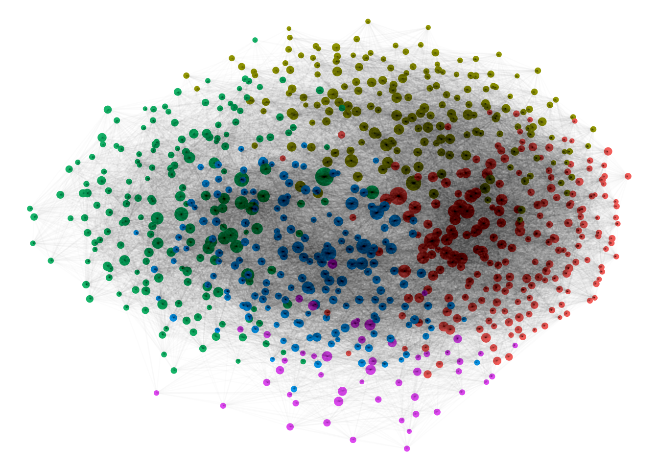
Co-Citation Networks from Letter Mentions: A Short Guide

Community Detection in a large academic co-citation network. A link is drawn (as a grey line) between two authors (as coloured circles) if they are both cited in the same paper. Data from: https://www.aminer.cn/citation

Figure 1: Community Detection in a large academic co-citation network. A link is drawn (as a grey line) between two authors (as coloured circles) if they are both cited in the same paper. Data from: https://www.aminer.cn/citation

This is an R Notebook: a document containing code and text. The source code is available in a GitHub repository. Download the folder and then open it with R-Studio to run the notebook yourself.

You’ll need a little bit of prior knowledge of R and the tidyverse to properly follow along, and maybe a basic understanding of the network analysis library igraph and network visualisation library ggraph to do any of your own analysis—if you want to try with your own dataset.

This post is the fifth in a series documenting some of the code and techniques we’ve been using on the Networking Archives project: you can read the earlier ones here

More info on the Github repository below

Co-Citation Networks and Historical Correspondence

A co-citation network is a network model which uses the principle that those mentioned (or cited) in the same document may share some kind of link. This kind of work has been widely used to understand, for example, the structure of communities of scholars—based on the principle that if two documents are often cited in the same document, they likely have some kind of semantic link. This is what is drawn in the network diagram above. Here it’s used just as a fancy illustration, but you could use it for analysis: for example, to check to see if the authors in the communities have any shared characteristics, or whether there are distinct communities of scholars or academic areas which repeatedly cite each other. Bipartite networks have also been used to understand ecological food webs - connecting animals which are all prey for the same predator, for example, or flowers pollinated by the same insect.

The method can also be used to understand other types of citations. One project, Six Degrees of Francis Bacon, uses co-citation of people in Oxford Dictionary of National Biography articles as a way of inferring some kind of likely social connection - again, based on the premise that if two people were repeatedly mentioned together in articles, they likely share some kind of link. Or, as done here, you could use co-citation to draw links between two individuals, if they are cited, or mentioned, in the same letter.

This article won’t go into much detail into the theory behind or benefits of co-citation networks. It’s intended as a brief tutorial on gathering data on people mentioned in letters, extracting it into a dataset, and visualising as a co-citation network.

It’s assuming you’re starting from scratch and either have a dataset of letter metadata (at the very least, a spreadsheet or letters with the names of senders and recipients, but probably with additional metadata such as dates and place of origin), or you intend to make one in which you’ll also record your people mentioned. If you already have people mentioned in some format in your dataset, you’ll need to make sure it fits exactly the format outlined below.

The tutorial will go through the following steps:

Collecting and then extracting the data from a simple spreadsheet.
Creating the bi-modal network (the term will be explained)
Projecting the bi-modal network to unimodal
Visualising the results.

Collecting and formatting the people mentioned data

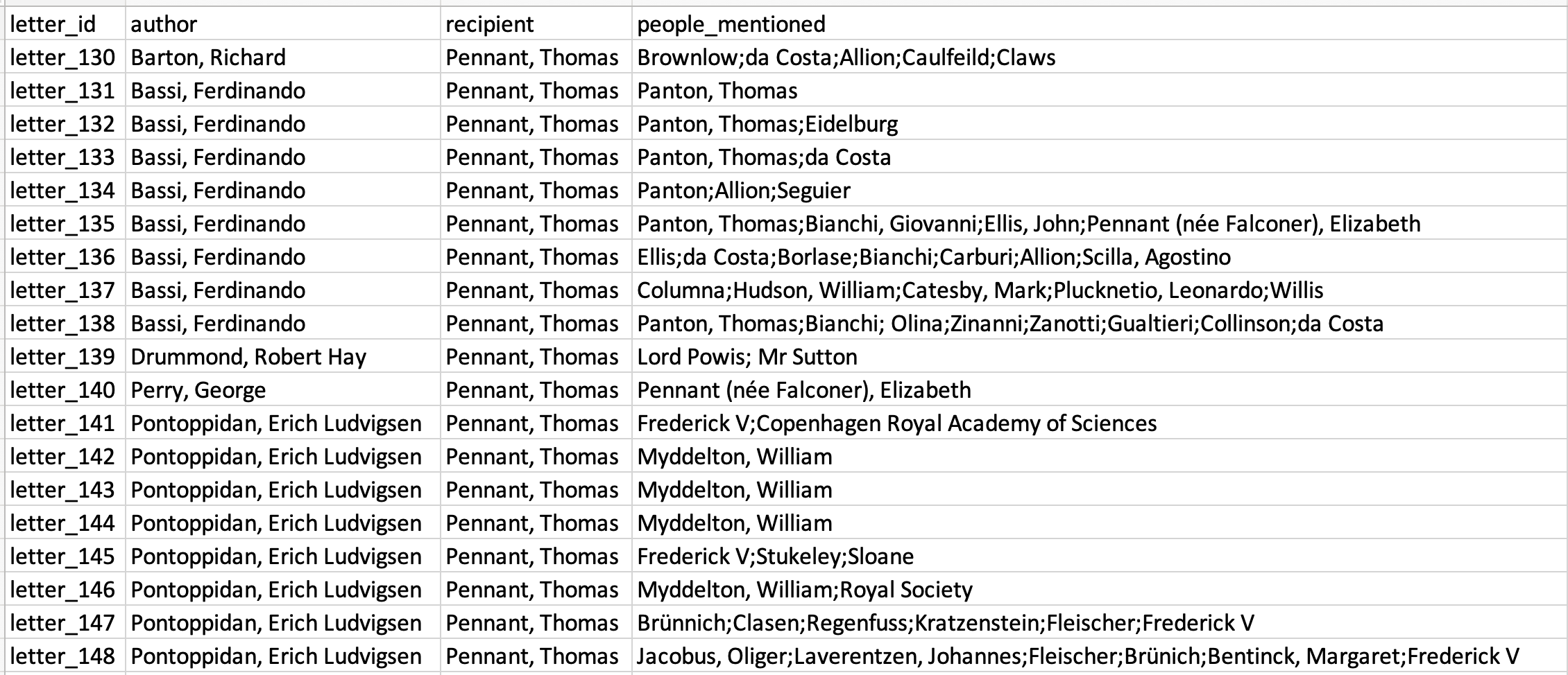
The first step is to read through letters and record the people mentioned in each of the letters. Letter metadata is most often recorded in a simple spreadsheet, with one row per letter, and a separate column for author, recipient, letter origin, and so forth. The easiest way to record people mentioned is in a separate column, with each separated by a semi-colon. There are a number of things to consider:

Is it possible that you’ll have several people with the same name? If so, you’ll need to come up with some way of distinguishing between them. What’s needed will depend a bit on the size of your dataset. If it is relatively small you could add birth and death dates, if you always have them, to each the people - so two John Smiths become John Smith (1700-1775) and John Smith (1655-1710). If you’re likely to have lots of names and adding dates to distinguish between them would be unwieldy, you could replace each person with a unique numerical code, with a separate ‘lookup table’.

Do your letters have unique identifiers? You need to identify each letter separately in order to build the co-citation network. If there’s not unique ID, add a simple system of sequential numbers as a first column in your letter dataset. In Excel or Google docs, this can be done just by typing in the first few numbers in a sequence, highlighting those you’ve done, and then clicking the little square in the bottom-right and dragging downwards.

Are you likely to have the same names occur in the author/recipient and person mentioned fields? If so, it’s important to make sure that people-mentioned names are distinguished from letter-author names (so if you have a John Smith author and a John Smith mentioned, you need to add a unique identifier to each to keep them separate - even if they are actually the same person!). You could, for example, add the word ’_mentioned’ to the end of each name in the person mentioned column.

For this example, I’ll assume that each name is unique, and that I can easily distinguish between each individual based only on their name. In a ‘real-world’ dataset, this is unlikely and I probably wouldn’t use simply the names.

Once you’ve decided on the appropriate system, create a new column called ‘people mentioned’ and record each person, followed by a semi-colon. It’s very important that the names used here are consistent - that you always refer to the person with the exact same name or code.

Once you’ve done this, import the data into R:

Load some libraries we’ll use:

library(tidyverse)
library(snakecase)

Load the sample mentions dataset (if you’ve downloaded the whole Github repo you should have this too). You could also swap in your own if you are confident it’s in the same format.

mentions = read_csv('mentions_example.csv')

Making the data ‘long’

In order to create the mention network, we need to transform the data. Most importantly, we need to create a table with two columns.

Column 1: the letter ID
Column 2: people mentioned

Crucially, instead of all the people mentioned per letter in one cell separated by a semi-colon, each person mentioned will have their own row, with the letter IDs duplicated as needed

So the first three letter records above would be transformed into the following:

We’ve made the data ‘longer’: see that letter 130, which had five people mentioned, is now transformed into five rows each with one person? This can be done with R and dplyr pretty easily.

The first step is to put each of the people mentioned in a separate column. For this we need to know the maximum number of columns will need, which can be done by counting the number of semi-colons and taking the maximum value, storing it as a variable called count.

count = max(str_count(mentions$people_mentioned, ";"), na.rm = T)

count

## [1] 7

Next, use the dplyr verb separate to create a new column for each name separated by a semi-colon. We tell separate to call the columns personmentioned1, personmentioned2, etc. with into = paste0("personmentioned", 1:count), sep = ';') This is where the variable called count comes in: we use it to specify how many columns separate needs to create so it can put each name in a separate one without cutting off the data.

people_mentioned_df = mentions %>% 
  separate(col = people_mentioned,
           into = paste0("personmentioned", 1:count), 
           sep = ';')

glimpse(people_mentioned_df)

## Rows: 19
## Columns: 10
## $ letter_id        <chr> "letter_130", "letter_131", "letter_132", "letter_13…
## $ author           <chr> "Barton, Richard", "Bassi, Ferdinando", "Bassi, Ferd…
## $ recipient        <chr> "Pennant, Thomas", "Pennant, Thomas", "Pennant, Thom…
## $ personmentioned1 <chr> "Brownlow", "Panton, Thomas", "Panton, Thomas", "Pan…
## $ personmentioned2 <chr> "da Costa", NA, "Eidelburg", "da Costa", "Allion", "…
## $ personmentioned3 <chr> "Allion", NA, NA, NA, "Seguier", "Ellis, John", "Bor…
## $ personmentioned4 <chr> "Caulfeild", NA, NA, NA, NA, "Pennant (née Falconer)…
## $ personmentioned5 <chr> "Claws", NA, NA, NA, NA, NA, "Carburi", "Willis", "Z…
## $ personmentioned6 <chr> NA, NA, NA, NA, NA, NA, "Allion", NA, "Gualtieri", N…
## $ personmentioned7 <chr> NA, NA, NA, NA, NA, NA, "Scilla, Agostino", NA, "Col…

This new dataset contains seven new columns, and each separate person mentioned is placed in one. If there are less than seven people mentioned, that column will have a NA value for that letter.

There’s one more important step before the data is in the format needed. Rather than having the people mentioned in columns running across from left to right, we need one letter column, and one person mentioned column (with letters repeated for multiple people, as above).

To do this use pivot_longer: another dplyr verb. This takes a selection of columns, and puts them into a ‘long’ format, with one value per row, rather than spread across mutiple columns.

names_to and values_to are names given to the new columns. We are going to throw away the names column in this case, so it doesn’t matter what we call it.
starts_with('personmentioned') is a useful function that will select all the columns that start with a given set of characters - we want it to take all the new columns that start with the words ‘personmentioned’ and put these into the correct format.

people_mentioned_longer = people_mentioned_df %>% 
  pivot_longer(names_to = 'inst', 
               values_to = 'person_mentioned', 
               starts_with('personmentioned'))

glimpse(people_mentioned_longer)

## Rows: 133
## Columns: 5
## $ letter_id        <chr> "letter_130", "letter_130", "letter_130", "letter_13…
## $ author           <chr> "Barton, Richard", "Barton, Richard", "Barton, Richa…
## $ recipient        <chr> "Pennant, Thomas", "Pennant, Thomas", "Pennant, Thom…
## $ inst             <chr> "personmentioned1", "personmentioned2", "personmenti…
## $ person_mentioned <chr> "Brownlow", "da Costa", "Allion", "Caulfeild", "Claw…

The last thing to do is to remove any NA values and select only the columns we’re interested in:

people_mentioned_longer = people_mentioned_longer %>%
  filter(!is.na(person_mentioned)) %>% 
  dplyr::select(letter_id, author, recipient, person_mentioned)

Bi-modal networks

At the heart of the co-citation network is a bi-modal or bipartite network. A standard network of correspondents is uni-modal - that is, the connections are between actors of the same type - any node can be a letter author or a letter writer. But networks can be between things of different types - for example, one can draw a network of authors connected to books, or actors to films, and so forth. It’s an established alternative method often used in network science. See, for example, Scott Weingart’s blog post (and tutorial) for more detail on this as a technique.

Even though it seems in this case both are the same type (people), for our purposes they are as different as authors and books. Two ‘people mentioned’ can never be directly connected. The resulting network needs to differentiate between the different types.

Constructing a Bi-modal network with ```igraph```

The first step is to load the igraph library (R’s most useful network analysis toolkit), get each unique combination of letter and person mentioned, and turn into a standard network graph using the igraph function graph_from_data_frame().

library(igraph)

edges = people_mentioned_longer %>% distinct(letter_id, person_mentioned)

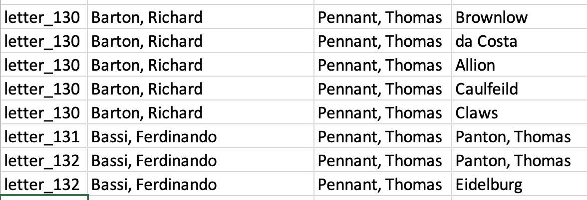
g <- graph_from_data_frame(edges, directed = F)

We can plot it using another package, ``ggraph()``. It shows a network where both types of nodes (people and letters) are directly connected.

library(ggraph)

ggraph(g) + 
  geom_node_point() + 
  geom_node_text(aes(label = name), size = 2.5)+ 
  geom_edge_link(alpha = .2) + theme_void()

What we are interested in is constructing a co-citation network: where links are inferred because of co-mention in the same letter. For this we need to turn the unimodal network into a bimodal one - one where the network software knows that the nodes are of two different types. This is done in igraph by adding a new attribute to the nodes in the network called type, which is either TRUE or FALSE depending on whether the node is from type A (letters) or B (authors).

It’s easy to do, because we know that if a node name is from column 1, it must be a letter, and if it’s column 2, it must be a person. This only works if the names used for both types are unique - if you were constructing a bi-modal network of, say, authors, connected to publishers, if the same person was both an author and a publisher, you’d need to distinguish between the type in the name.

V(g)$name %in% people_mentioned_longer$person_mentioned looks horrible but returns a vector of TRUE or FALSE values, depending on whether or not a name is in the person_mentioned column. V(g) selects the vertices (nodes) in the graph we’ve created, and V(g)$type = creates a new attribute for these vertices and then stores the TRUE/FALSE vector in that attribute.

V(g)$type = V(g)$name %in% people_mentioned_longer$person_mentioned

Now letters and people are distinguished. This can be drawn again using ggraph:

ggraph(g) + 
  geom_node_point(aes(fill = type), size = 4, pch = 21, color = 'black') +
  geom_node_text(aes(label = name), size = 2, repel = T)+ 
  geom_edge_link(alpha = .2)+ 
  theme_void()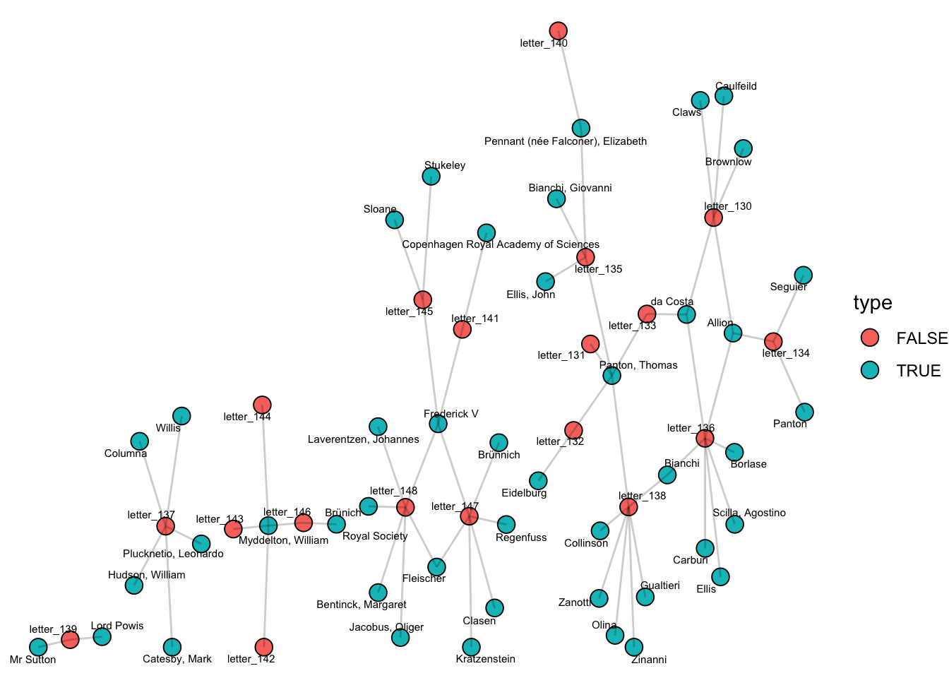

Igraph has a layout specifically for these types of networks called ‘as_bipartite’, which separates out the two types, and tried to cluster them together based on their connections to the other type (though I’m not so sure it is much use here):

ggraph(g, 'as_bipartite') + 
  geom_node_point(aes(fill = type), size = 4, pch = 21, color = 'black') + 
  geom_node_text(aes(label = name), size = 2, repel = T)+ 
  geom_edge_link(alpha = .2)+ theme_void()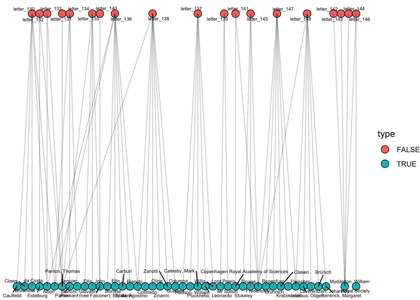

Project the bi-modal network

The final step is the project the network. This is a process of collapsing the bi-modal network into one of its types - with links (or edges) drawn between nodes based on their connection to the other type. A link is drawn if both nodes were connected to the other type.

The igraph function bipartite_projection() takes care of all this. It will create two new graphs - one where letters are connected if they both mention the same individual (not so useful) and one where people are connected if they are both mentioned in the same letter (more useful). The new graphs are stored as a list: list elements can be accessed using [[1]] or [[2]].

projections = bipartite_projection(g)

First the letter network:

projections[[1]] %>% 
  ggraph() + 
  geom_node_point()+ 
  geom_node_text(aes(label = name))  + 
  geom_edge_link(alpha = .1) + theme_void()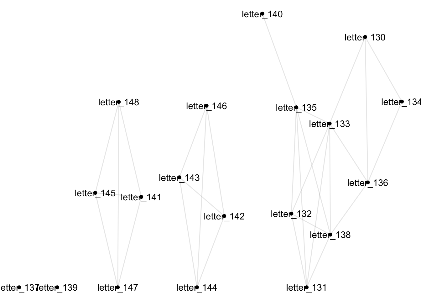

In this case, I would struggle to see how the collapsed letter network, with letters connected if the same person is mentioned within them, could be useful. That may not always be true though, depending on the type of document and the specific research question. You could imagine a research question which looked for connections between journal articles based on their citations, for example.

Next the people, sized by their total connections (degree):

V(g)$degree = degree(g)

V(projections[[2]])$degree = degree(projections[[2]])
projections[[2]] %>% 
  ggraph() + 
  geom_node_point(aes(size = degree), size = 4, pch = 21, fill = 'lightblue', color = 'black')+ 
  geom_node_text(aes(label = name), repel = T, size= 2)  + 
  geom_edge_link(alpha = .1) + 
  scale_size_area()+ 
  theme_void()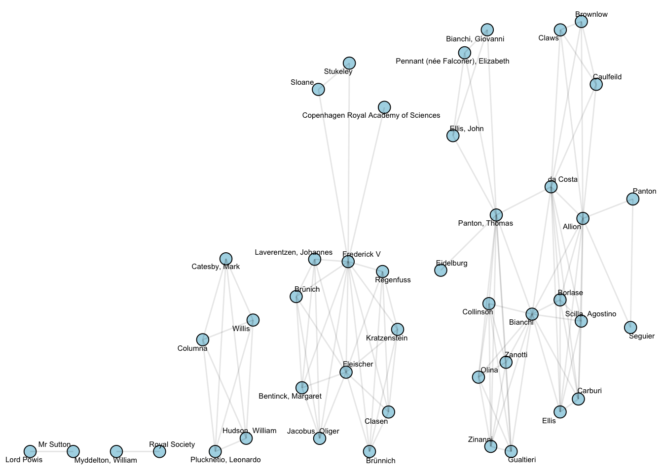

What to do with it?

Once you have this projected network, it can be treated as any other network graph. All the same metrics (centrality measures such as degree, community detection, and so forth) can all be calculated as if it was a regular network. Whether you should or not is another question, however. You should think carefully about whether the results are meaningful for your particular dataset- it may be more difficult to interpret centrality in a co-citation network than in a regular one, for example. For one thing, you’re likely to get incredibly dense networks once you project to a unimodal, which makes them hard to directly compare to a regular correspondence network. Scott Weingart discusses these questions in detail in his blog post on bi-modal networks.

Co-Citation Networks from Letter Mentions: A Short Guide

Co-Citation Networks and Historical Correspondence

Collecting and formatting the people mentioned data

Making the data ‘long’

What to do with it?

Further reading

More info on this document

Co-Citation Networks from Letter Mentions: A Short Guide

Co-Citation Networks and Historical Correspondence

Collecting and formatting the people mentioned data

Making the data ‘long’

Bi-modal networks

Constructing a Bi-modal network with ``igraph``

Project the bi-modal network

What to do with it?

Further reading

More info on this document

Constructing a Bi-modal network with ```igraph```